A Framework for Modeling Cyber-Human Systems ..... a set of CHS measures of value, what is the best configu- ration .... spent on IT support, e.g., the help desk.
The Multiple-Asymmetric-Utility System Model: A Framework for Modeling Cyber-Human Systems Douglas Eskins and William H. Sanders Information Trust Institute, Coordinated Science Laboratory, and Department of Electrical and Computer Engineering University of Illinois at Urbana-Champaign {eskins1, whs}@illinois.edu
Abstract—Traditional cyber security modeling approaches either do not explicitly consider system participants or assume a fixed set of participant behaviors that are independent of the system. Increasingly, accumulated cyber security data indicate that system participants can play an important role in the creation or elimination of cyber security vulnerabilities. Thus, there is a need for cyber security analysis tools that take into account the actions and decisions of human participants. In this paper, we present a modeling approach for quantifying how participant decisions can affect system security. Specifically, we introduce a definition of a cyber-human system (CHS) and its elements; the opportunity-willingness-capability (OWC) ontology for classifying CHS elements with respect to system tasks; the human decision point (HDP) as a first-class system model element; and the multiple-asymmetric-utility system modeling framework for evaluating the effects of HDPs on a CHS. This modeling approach provides a structured and quantitative means of analyzing cyber security problems whose outcomes are influenced by human-system interactions. Keywords-Quantitative Security Model, State-based Security Model, Cyber-Human Systems, Human Decision Points
I. I NTRODUCTION Traditional approaches to cyber security evaluation either do not explicitly consider human participants “within” the system or view participants as a set of static properties that are independent of the system. In this paper, we discuss a new approach that explicitly considers human participants as integral system elements. Here cyber security evaluation means the assessment of security properties related to the prevention of, detection of, and response to attacks on any complex system in which computers play a key role. Many cyber systems, by design or implication, involve human participants. We shall refer to systems of this kind as cyber-human systems (CHSs) (see Section II) and propose that any model of a CHS is incomplete without due consideration of its human participants. CHSs are increasingly important within organizations, and thus, the security concerns surrounding these types of systems, i.e., CHS security, are also increasingly important. Typically, CHS security only evaluates physical devices, e.g., firewalls; software, e.g., anti-virus software; or administrative controls (ACs), e.g., security policies and procedures. Many ACs, however, depend upon the compliance of system participants, and it is common when evaluating such controls
to assume that participants will always comply with the rules. We believe that this assumption is erroneous and that the willingness of participants to comply with ACs can and will vary, depending on factors such as the design of the controls, the state of the system, and the incentives for participants. The failure of participants to comply with ACs can lead to serious security vulnerabilities that are not accounted for in traditional CHS security evaluation methods. At the core of this issue is the difference in goals between individuals and the organization [1] [2]. We propose to study the following problems. 1) How can modeling the difference between participant goals and other goals provide insights into human and system performance? 2) What can models of this type reveal about unexpected system performance or a persistent failure to meet goals? 3) Finally, how can explicit modeling of human decisions provide better analysis and configuration management tools than traditional CHS security evaluation approaches do? The contributions of this paper are the following: • the introduction of the CHS model and its basic elements, • the definition of the opportunity-willingness-capability ontology, • the definition of the human decision point, and • the introduction of the multiple-asymmetric-utility system modeling framework as a tool for analyzing cyberhuman systems. Specifically, we present a modeling approach for quantifying how humans “within” a CHS can affect the system security state. Our approach is to explicitly model human behaviors as integral system elements and measure how human decisions affect system state and vice versa. We begin in Section II by defining our concept of the CHS model and its four basic element types. In Section III we define the basic opportunity-willingness-capability (OWC) ontology and describe how it may be applied to describe performance conditions for CHS task elements. In Section IV we describe how certain key tasks can be identified as human decision points (HDPs). In Section V we present the multiple-asymmetric-utility system (MAUS) framework, and in Section VI we discuss our solution method using
MAUS. In Section VII we apply the MAUS framework to an example CHS and show how MAUS may be used 1) to validate HDPs within a given CHS; 2) to quantify the significance of human decisions relative to security goals; 3) to quantify the divergence between expected human behavior and ideal human behavior; and 4) to provide decision tools for system design and configuration. We conclude in Section VIII. II. T HE C YBER -H UMAN S YSTEM M ODEL To describe how we model the effects of human behaviors, and especially human decisions, on a system, we will first describe our modeling view of the CHS. That is, we will describe how a CHS may be decomposed into model elements. A running example will be presented in this and following sections to add clarity. As described in the introduction, a CHS is any system in which computers and humans are key elements. Examples of such systems include a typical business or academic IT infrastructure, a manufacturing process control system, or something as simple as a cell phone and its user. For each of these examples, a model may be created in which humans perform tasks using the CHS for the achievement of goals.
Figure 1.
Cyber-Human System Element Types
A. Cyber-Human System Element Types The first step in constructing such a model is the definition of our CHS of interest. Our system view divides CHS elements into four types: “components,” “participants,” “processes,” and “tasks.” We assume that all relevant CHS properties can be represented using these element types. Components are the physical objects used to build the system. For example, in a business IT infrastructure, the set of components would include system servers, network connections, workstations, and software. Participants are the entities that perform actions within a system. In most cases, participants are humans, but a nonhuman entity, such as an automatic security function, may also be considered a participant. Processes define how the system is used and are usually associated with some purpose or goal. For example, a process in a business IT system might define how Internet sales are credited to accounts, with a goal of 100% transaction accuracy. In Section V-B we will describe utility functions as ways of measuring the achievement of goals. A process defines a flow or ordering of tasks, as described next. Tasks are the units of action within a system. Using terminology similar to that of [3], we define a task as an atomic unit of work that is carried out by a resource, where a resource is one or more participants. A compact definition showing the relationship among CHS elements is “a process is a defined flow of tasks performed by one or more participants using system components.” In modeling terms, this means that state changes can only occur as the result of task performance, and model
Figure 2.
Example Cyber-Human System
elements can only affect each other via some task. Figure 1 illustrates this relationship. For example, a participant can only change the state of a process via a related task. Running Example: USB Stick Usage as a CHS. Based on a study of the security aspects of USB stick usage [1], we use as our running example the USB Stick Usage CHS (Figure 2). Here, the CHS is a business environment where company representatives use USB sticks to store sensitive data. USB sticks are used in various environments. These environments include the employee workstation, company meetings, visits to business clients, the employee’s home, and transit between locations. Each environment has tasks and risks associated with the USB stick. Company security policy states that sensitive information stored on USB sticks must be encrypted. However, employees can choose whether to follow this policy or not. Periodically the company performs a security scan on USB sticks for unencrypted sensitive data and punishes employees who have violated the security policy. The company also provides IT support to employees for USB stick issues. The IT department has a fixed budget that is allocated between IT support and security scans. Company IT security goals include measures of USB data availability and confidentiality. Successful transfers of USB data positively affect availability. Loss or compromise of USB data negatively affects confidentiality.
Additionally, participants have their own goals. They value the availability of USB data but seek to avoid embarrassment when they cannot access data, frustration with IT support failures, and management sanctions for violating the security policy. Below we list some representative CHS elements grouped by their element types for this example system. • Components: USB stick, encryption software, business IT system, and various environments. • Participants: business representative and a software routine to perform an automated security scan. • Processes: transferring company data to and from the USB stick, conducting client visits, checking for compliance with security policies, and moving between physical locations. • Tasks: encrypting USB data, reading encrypted USB data, and utilizing IT support. Now that the basic elements of the CHS model have been defined, we will next describe how they can be grouped relative to CHS tasks.
Figure 3.
OWC Ontology
III. O PPORTUNITY-W ILLINGNESS -C APABILITY Given that all actions within a system occur as tasks (see Section II-A), it is necessary to define what system states lead to task performance. We do this by associating sets of CHS elements with each task using a formal naming system, the opportunity-willingness-capability (OWC) ontology. Simply put, the OWC ontology classifies a set of CHS elements on which task performance is conditioned. This classification is described below. A. Task Performance Generally, task performance may lead to several outcomes. However, for simplicity, we define a task in terms of binary outcomes: “proper” or “not proper” performance. Here proper performance means the achievement of some desirable end state. We believe this is reasonable, as any task featuring multiple outcomes can be decomposed into a set of binary tasks. Running Example: Task. The task selected for our running example is Encrypt USB Data (EUD). This task is part of the process for writing new USB data. It is performed properly if the data are encrypted and not performed properly otherwise. As shown in Figure 3, for a task to have the potential to be properly performed, the current model state must be the intersection of possible model states for which OWC (as described next) can be evaluated as true. B. Opportunity Opportunity captures the idea of prerequisites for task performance. In terms of our system model, opportunity is related to a set of state variables required to attempt a task. These are known as the task-specific set of opportunity elements (OEs). OEs may be drawn in any combination from
Figure 4.
A Task’s OWC Defines Sets of System Elements
CHS elements (see Figure 4). For each task an opportunity function (fO ) is defined that maps OE states to {0, 1}. A 1 indicates that there is opportunity for task performance. Running Example: Opportunity Elements (OE). Per our running example, we will list the OEs for the task EUD using the following notation: ElementLabel.state = ElementState The opportunity elements for EUD are the set OE = {U, E, L}, where U represents the USB stick, E represents the encryption software, and L represents the participant location. The possible OE states are: • • •
U.state ∈ {participant possesses (P ), participant does not possess (N P )} E.state ∈ {available (A), not available (N A)} L.state ∈ {at workstation (W ), in transit (T ), using personal computer (P )}
Running Example: Opportunity Function (fO ). fO is a Boolean equation that uses as inputs the task-specific OEs above and evaluates to 1 or 0 (see Equation 1). fO = (U.state == P )(E.state == A)(L.state == W ) (1)
If fO is evaluated as 1, then the opportunity for task performance exists. C. Willingness Willingness captures the desire of the participant to perform a task and thus is only applicable to tasks performed by humans. In terms of our system model, willingness is related to a set of state variables that may influence a participant’s desire to perform a task; they are called the task-specific set of willingness elements (WEs). Much like the opportunity function, a willingness function (fW ) is defined that maps the set of WE states to {0, 1}. However, instead of being deterministic, fW is stochastic. That is, fW maps the set of WEs to a random variable from which the willingness probability (WP), i.e., the probability that the participant is willing to perform the task, is determined. In general, fW can map to many random variables; however, for our initial approach, we used a Bernoulli random variable with a fixed WP to define an fW that is independent of model state. Running Example: Willingness Elements (WEs). In our running example, there are no WEs. See Section V for more details. Running Example: Willingness Function (fW ). The fW used in our example is a simple Bernoulli trial in which the probability of success is simply the willingness probability (WP). (See Equation 2.) Success here means that the participant is willing to attempt the task. fW = Bernoulli(W P )
(2)
D. Capability Capability captures the idea that a participant, given opportunity and willingness, can properly perform a task only some of the time. In terms of our system model, capability is related to a set of state variables that may influence a participant’s ability to perform a task; they are known as the task-specific set of capability elements (CEs). Like fW , a capability function (fC ) stochastically maps the set of CE states to {0, 1} via a function of random variables. One way of interpreting this is that some system states might produce a higher probability of capability, e.g., evaluation of fC as 1, than other states. The capability function is in general complex, so to simplify matters, we defined fC as a Bernoulli random variable in which capability probability (CP), or the probability that capability will exist, is the product of n independent capability transfer functions (CTFs) (see Equation 3). Each CTF maps a subset of CEs to an independent Bernoulli probability of success. As an example, see the CTF shown in Figure 5 which maps the CE level of training to a probability of successful task performance. The CTF product, CP, represents the overall Bernoulli probability that capability exists. Note that we assume that the set of CEs can be divided into independent (relative to that task) subsets.
Figure 5.
Example of a CTF That Maps Training to Performance
CP = CT F1 × CT F2 × ... × CT Fn
(3)
Running Example: Capability Elements (CEs). In our running example, CEs are those model elements that affect how likely it is that the task, encrypt USB data, will be properly performed. The CEs for this task form the set CE = {T, H}, where T represents the level of training received on the use of the encryption software and H represents the availability of IT support. In general, CE states can be drawn from a set of discrete values or even a continuous interval. We will define them here as below: • T.state ∈ {0.2, 0.8} • H.state ∈ {Available, Not Available} Running Example: Capability Function (fC ). For this example, CP = CT FT × CT FH , where CT Fi represents the CTF for CE i. The resulting fC maps {T × H} to {0, 1} (see Equation 4). fC = Bernoulli(CP )
(4)
In summary, the OWC ontology is useful in two ways. First, during the model definition phase, the OWC ontology provides a structured way of defining and grouping model elements for each task. For example, to model a process, the process is typically first decomposed into an ordered arrangement of tasks [4] [5]. While performing this decomposition, the analyst can directly define state variables by listing the OWC elements associated with each task. Second, during the model execution phase, only those elements defined by the OWC ontology are evaluated for a given task. This contributes to execution efficiency. IV. H UMAN D ECISION P OINTS (HDP S ) Now that we have defined our model as described in Section II and linked each task to associated OWC conditions as described in Section III, we are ready to introduce a special type of task, the human decision point (HDP). Consider first an abstract view of a system model as a set of states and a set of events that define transitions between
states [6]. From this viewpoint, a task can be regarded as two possible events, proper or not-proper task performance. The outcome of the task is dependent on the current states of the task-specific OWC elements. From a modeling point of view, an HDP represents a point in the execution of the model in which the next state depends, at least in part, on a human decision. Given that our model consists of binary tasks, some tasks can be viewed as decisions between two actions. That is, given that a participant has the opportunity and capability, the participant must also decide, i.e., be willing, to properly perform the task. Thus, it is straightforward to define an HDP as a task performed by a human participant for whom willingness is not always true. A second criterion for an HDP is that it must be significant relative to a utility function, as described in Section V. That is, we define an HDP not only by whether or not a human participant makes a decision, but also by how significant that decision is to the system. Running Example: HDPs. In our running example, we wish to select for special evaluation a task for which human decisions are both relevant (e.g., the participant is allowed to make a decision) and significant (e.g., affects a utility value) to the USB Stick Usage CHS. In previous examples, we defined the task EUD. Recall that system security policy states that sensitive USB data should always be encrypted; however, the participant may choose whether or not to comply with the stated policy. Because the performance of this task is dependent upon the participant’s willingness to encrypt data, we shall also select the task EUD to be our HDP of interest. It is not immediately obvious that the EUD task will also have a significant effect on a utility function value. However, because the task directly affects both the security and participant utility functions via data availability, it seems to be a good candidate for analysis. By looking at the results in Section VII, we shall see that task EUD does indeed have a significant effect on the participant and security utility function values and thus also meets the second criterion for an HDP. In the next section, we will present the modeling framework used to arrive at these results. V. T HE M ULTIPLE -A SYMMETRIC -U TILITY S YSTEM (MAUS) M ODELING F RAMEWORK Given the above modeling concepts, we introduce a modeling structure for applying them called the multipleasymmetric-utility system (MAUS) framework, shown in Figure 6. MAUS includes not only the system model, but also a structured way of running many experiments and consolidating results. It has four basic parts: 1) a system model, 2) a set of utility functions, 3) a set of system configurations, and 4) a range of willingness probabilities (WPs) for each HDP in the system model.
Figure 6.
Figure 7.
MAUS Framework
Building the MAUS Framework
We set the stage for describing MAUS with the following problem. Given a CHS, a set of CHS configurations, and a set of CHS measures of value, what is the best configuration? MAUS will help us answer questions of this type. Figure 7 summarizes the basic process of building a MAUS framework as described in the following sections. A. System Model First, a system model is defined in terms of CHS elements as described in Section II. Next, the task conditions are defined in terms of the OWC ontology described in Section III. Once utility functions for each domain of interest are defined as described in Section V-B, appropriate tasks may be identified as HDPs, as described in Section IV. The set of CHS elements along with task conditions and HDPs makes up the system model used by MAUS (Figure 6). Of course, what we have described so far is a “conceptual” system model and may be implemented using any number of formalisms. For the results presented in this paper, we implemented the model using the stochastic activity network formalism in M¨obius [7]. Once implemented, the system model must be solved for each experimental configuration as described in Section V-C
over a set of possible WPs described in Section V-D. Due to the complexity of the model, simulation was used to obtain the results presented in Section VII. During model simulation, utility functions were applied to measure and record system values, as described in the next section. B. Utility Functions Utility functions define measures of value for a given system state during simulation. Much like OWC functions, utility functions use a collection of state variables, called utility elements (UEs), to calculate domain-specific values. Domain-specific here references a given viewpoint, e.g., the viewpoint of a system participant or the IT security manager. MAUS uses multiple asymmetric utility function groups, one for each domain of interest, including a utility group for system participants. Though these domains may not be mutually exclusive, they can still be very different, and this difference is key to our solution method. That is, the decisions of participants, which influence the system state, are made by considering participant utility (not security utility). Thus, to accurately evaluate a system, multiple utility measures are used both to predict the decisions of participants and to assess the system state. For now, let us consider two basic utility function groups: participant and security. The participant utility (PU) function group measures the values of state variables, e.g., participant utility elements (PUEs), relative to a participant. Many different types of measures are possible, including instantaneous and timeaveraged values. In M¨obius, these measures are called reward functions and can be almost arbitrarily complex. See [6] and [7] for greater detail on reward functions. Similarly, the security utility (SU) function group measures the values of state variables, e.g., security utility elements (SUEs) relative to a set of security metrics or goals. Examples might include measures of data integrity, confidentiality, and availability. Because MAUS considers utility functions separately from the system model, the addition of utility function groups is straightforward. As an example, Figure 6 includes a business utility function group that might be added to measure a business metric such as the cost of providing IT support. Running Example: Utility Functions. The PU function (fP U ) is a weighted linear combination of four PUEs (see Equation 5): successful data transfers, S; embarrassments, E; management dings, M ; and negative support experiences, N. fP U (S, E, M, N ) = γ1 S − (γ2 E + γ3 M + γ4 N )
(5)
S reflects the number of times that data were successfully transferred by the participant. This is considered a reward and adds positive value to fP U .
E represents the number of times a business representative was unable to retrieve data and was embarrassed. M represents the number of times a security scan discovered unencrypted sensitive USB data and a “black” mark was placed on the employee’s record. N represents negative IT support experiences. E, M , and N are considered penalties and have a negative effect on fP U . Each PUE has an associated weight (γi ) reflecting its importance to the overall PU value. These values are determined by system stakeholders when the utility functions are defined as part of the MAUS definition phase. The SU function (fSU ) for our example is a weighted linear combination (see Equation 6) of confidentiality, C, and availability, A. fSU (C, A) = α(A − βC)
(6)
Availability is defined as the average number of successful data transfers performed by a participant each year. Confidentiality is defined as a weighted linear combination of data exposure events and amount of data exposed. A data exposure event occurs when unencrypted sensitive USB data are exposed to an unauthorized person. The weights α and β represent the relative importance of C and A to fSU . It should be noted here that the utility functions defined in this paper were selected during a study of the security aspects of USB stick usage [1]. The intent of the MAUS framework is to provide a rationale and method for using utility functions to study CHSs. It is not a means of validation for utility functions, and any utility function applied to the MAUS framework should be subject to domain-specific validation prior to use. Next, given a defined system model and a set of utility functions, a set of initial conditions must be defined via the system configuration. C. System Configuration A system configuration (Sys Conf) is the set of initial conditions for which the system model will be solved. Typically, when referring to a given Sys Conf, we will only describe those items that will be varied for the purposes of the experiment. It should be noted that the initial conditions for most CHS elements are fixed, as they either do not frequently change (like hardware used by the system) or are physical properties over which the system manager has no control. As an example, let us suppose that a given CHS model requires that initial values be defined for the set of n elements, E = {e1 , e2 , ..., en }, where each element, ei , is itself a set of possible element state values. We define the set of Sys Conf elements, EC ⊂ E, as the subset of elements in E that will be varied between experimental series. If EC = {e1 , e2 , ..., em }, we define C, the set of all possible Sys Confs, as the set of all possible states of the elements
in EC or C = {e1 × e2 × ... × em }. A specific Sys Conf, ci , is thus an element in C. Each Sys Conf, ci , defines a corresponding experimental series, i. Each experiment in an experimental series is a system solution obtained using a fixed Sys Conf and WP. See Section VI for more details. Running Example: System Configuration. In our example, the system manager can control the portion of the IT budget spent on IT support, e.g., the help desk. The remaining budget is spent on enforcement of IT security policies. Since the portion of the IT budget spent on IT support or enforcement is the only aspect of Sys Conf that we are studying, i.e., it is the only initial Sys Conf value we are varying, each Sys Conf is characterized solely by the portion of the IT budget spent on IT support. Thus, C = {ci ∈ [0, 1]},
(7)
where C is the set of all possible Sys Confs and each ci defines an experimental series with a fixed portion of the IT budget spent on support. Because the underlying system model is stochastic, an individual experiment must be repeated many times to build sets of results that have the desired confidence intervals (at least with respect to simulation results, as discussed in Section V-A). Each repetition of an experiment is known as an experimental run, and the number of experimental runs required to achieve the specified accuracy for a given experiment will vary based upon the complexity of the model and the type of measures collected. In the MAUS framework, each experiment is associated with a fixed WP value as described in the next section. D. Willingness Probability For each experiment, a WP, as discussed in Section III-C, is set for each HDP within the system. As stated previously, WP generally will be one of many state-based inputs to fW . However, for these experiments, we have chosen WP by itself to represent a Bernoulli probability of a participant’s willingness to properly perform at an HDP. For example, if WP is set to 0.30, at each opportunity to perform the task, there is a 30% probability that the participant will actually choose to attempt proper task performance. For each HDP, a set of WP values must be selected from the interval [0, 1] to represent possible expected values for that decision. It is the goal of the MAUS framework to determine over an experimental series which value of WP maximizes fP U as described in the next section. VI. S OLUTION M ETHOD Now that we have defined all the parts of the MAUS modeling framework, in this section we apply them using an iterative solution method and an assumption regarding human decision-making. Then we provide examples of useful results that can be obtained using MAUS.
Figure 8.
Single HDP Example
The MAUS modeling framework uses the following method for solving a set of experimental series: for each fixed Sys Conf, an experimental series (as discussed in Section V-C) is solved in which WP for each HDP is varied from 0.0 to 1.0. Each experiment (within an experimental series) consists of solving the system model for a fixed Sys Conf and a fixed WP. Utility measures are extracted during each experiment and stored. When all experiments in the series are complete, the process is repeated for the next Sys Conf until all Sys Confs have been solved. It is our explicit assumption here that the expected value of a given human decision, i.e., the expected WP that a participant will attempt task performance, can be estimated by choosing the experimental run with the highest participant utility value. That is, on average, a participant will make the decision that provides the most value to him or her based on the provided system state. This decision may not provide the greatest utility for other measures within the system. Thus, because human decisions are part of the system model state, other utility measures must be experimentally derived using the expected value of WP for each HDP within the system. This solution method is illustrated for a single experimental series in Figure 8. It should be noted that this method is not easily scalable. The solution space that must be explored becomes prohibitively large as the number of HDPs grows beyond a small number. Here we consider a simple case in which MAUS is used to solve for the expected WP of a single HDP and a single SU value. Note that the highest participant utility is achieved at approximately a 40% WP. That value is considered the expected WP for this configuration, and thus the SU value must be calculated using this expected WP, i.e., the human decision probability that characterizes actual system performance. We refer to this SU value as the effective SU value. We also note that many current security metrics assume 100% participant compliance with administrative security policy, and we shall refer to this SU value as the ideal SU value. We assert that the effective SU value is a more accurate
representation of security performance than the ideal SU value is, because it accounts for the effects of human decisions. The difference between the ideal and effective SU values is the SU divergence (SUD). System performance metrics utilizing concepts such as the SUD, when calculated over a set of possible Sys Confs, can provide security managers with intuitive tools for managing Sys Confs. For example, in Section VII-B we use SUD to provide a simple graphical tool for selecting a configuration with security performance closest to the “ideal,” i.e., a SUD closest to zero. An example pseudocode for using MAUS to solve a system of this type is given in Algorithm 1. Note that for a fixed Sys Conf, ci , the system model (SYS) is iteratively solved for a range of WPs from 0.0 to 1.0. A participant utility (PU) value is recorded for each solution, i.e., P UW P . The WP that results in the highest PU value, i.e., MaxPU, determines the expected WP, i.e., ExpectedWP, value and is used to solve the system model for the effective SU value, i.e., EffectiveSU. Algorithm 1 MAUS Solution Method 1: ci ← SysConfig for Experiment 2: ExpectedWP ← 0 3: MaxPU ← 0 4: for W P = 0.0 to 1.0 do 5: P UW P ←SYS(ci , WP) 6: if P UW P ≥MaxPU then 7: ExpectedWP ← W P 8: MaxPU ← P UW P 9: end if 10: W P ← W P + 0.1 11: end for 12: EffectiveSU ← SYS (ci , ExpectedWP) VII. RUNNING E XAMPLE : A PPLICATION OF MAUS TO USB U SAGE E XAMPLE In this section we will provide some results from using MAUS to analyze our running example. As stated previously, the example is based upon the USB costs and benefits study undertaken in [1] (discussed in Section II-A) and examines the effects of IT security investment decisions on administrative security policy compliance and SU values. Recall that spending in the IT security budget can take two forms: IT support or IT security policy enforcement. The annual security investment is fixed and can be spent to improve the IT support desk or to increase participant monitoring. Spending on IT support increases the probability that IT support will be successful, perhaps as the result of hiring more support staff or improved customer service. Monitoring is used to check USB devices periodically for unencrypted sensitive data (a violation of the security policy that is punished with a management ding, M ). Increasing the
Figure 9.
IT Support Budget Portion Study
investment in monitoring results in more frequent checks of USB devices. The portion of the total IT budget spent on either the IT support desk or monitoring is varied for each configuration. For example, a particular configuration might spend 30 percent of the budget on monitoring and the remaining 70 percent on IT support. To produce the results in this section, a range of Sys Confs, e.g., the portion of the IT security budget that was spent on support, was examined, and the expected WP (i.e., the probability the participant will make the decision to encrypt USB data per the security policy) was calculated for each configuration. Results are presented first as raw participant utility values for each configuration, and next as plots of the expected WP for each configuration. A. Finding the Expected Willingness Probability We examined six Sys Confs (see Figure 9) by varying the portion of the annual security investment spent on IT support, using values between 0.0 and 1.0. For each configuration, the probability that the participant would comply with the security policy and encrypt sensitive data, namely the WP for the Encrypt USB Data HDP, was varied from 0.0 to 1.0. A corresponding PU value was calculated for each WP value. By the assumptions of the MAUS framework, the WP corresponding to the highest PU value represents the expected WP for that Sys Conf. We should note here that many experts believe that human beings do not strictly make utility-maximizing decisions [8]. We address these concerns with two points. First, MAUS is used to find the expected value of a decision over time, not calculate an individual decision. We believe this can provide at the very least the general tendency of human behavior relative to the system. Second, the current MAUS framework can be used to evaluate more complex human decision models by adding new utility functions and modifying the basic assumption of the solution method.
Figure 10.
USB Usage Willingness Transfer Function
Several interesting observations can be made from the results. First, note from Figure 9 that when all of the security investment is spent on monitoring, i.e., a completely punitive strategy corresponding to a Sys Conf with an IT support budget portion of 0.0, the highest PU value occurs at an expected WP of 0.0. This indicates that participants find it more rewarding not to follow the security policy even when punishment is highest. Why? The results indicate that without good IT support, encryption becomes so difficult that it is actually more beneficial for participants to transfer unencrypted data and risk punishment than to attempt encryption. The value of increased successful data transfers (S), fewer embarrassments in front of clients (E), and fewer negative support experiences (N ), outweighs the increased risk of management dings (M ). The results from the opposite case, i.e., the case in which all the security investment is spent on IT support (corresponding to a Sys Conf with an IT support budget portion of 1.0), can be understood in a similar way. Here, the expected WP, i.e., the expected compliance with the security policy, is also zero, because the risk of management dings (M ) is low (due to no monitoring) compared to increases in successful data transfers (S) and decreases in embarrassments (E) and negative support experiences (N ) that result from not using encryption. B. Derived Functions Above, we described how a given Sys Conf may be solved for an expected WP. In this section, we will describe two example functions of expected WP that may be used for configuration decisions: the willingness transfer function and the SU divergence ratio. Willingness Transfer Function Figure 10 plots the expected WP and SU values for each Sys Conf. The graph shows how participant behavior (e.g., the expected WP for complying with the administrative security policy) varies with Sys Conf (e.g., the portion of the IT security budget that is spent on IT support). The
graph also shows the effect participant behavior has on the resultant system SU value. Figure 10 illustrates an example of a system willingness transfer function. It represents a decision-making tool for security managers and allows them to take human behavior into account when selecting the best Sys Conf. Note that the highest levels of compliance are actually achieved when spending is approximately evenly divided between IT support and monitoring. That seemingly provides the right mix of rewards and punishments for this particular system. Of course, achieving the highest compliance with security policy is not always the same as achieving the highest SU value. Figure 10 indicates that the configurations with the highest participant compliance (configurations with an IT support budget of 0.4 to 0.6) actually correspond to the lowest SU values. That demonstrates the kind of counterintuitive result that a MAUS quantitative analysis can reveal. In this case, compliance with the security policy actually has a negative effect on the company IT security metric. In fact, the highest SU values are achieved by allocating the security investment budget all on monitoring or all on IT support. Those configurations, as discussed before, also happen to be those that result in the lowest participant compliance with administrative security policy. Why? It is most likely due to the importance of USB data availability to both the participant and SU function values. Increased availability results in higher participant and security utility scores. Thus, we achieve the counterintuitive result that lower participant compliance with security policy actually results in “better” security performance. Since the system security value is measured by the SU function, a system manager would presumably select a configuration to maximize the value of SU, not participant compliance. Understanding how system participants are expected to behave and how that behavior may affect overall system SU values becomes one more tool for system managers to use in making Sys Conf decisions. Security Utility Divergence Ratio A security manger may also wish to quantify how the SU value for a given Sys Conf varies from its ideal value, i.e., the value achieved at 100% participant compliance with security policy. Using the idea of SU divergence developed in Section VI, we can create a simple metric called the SU divergence ratio (SUDR) calculated relative to the highest SU value (see Equation 8) and plot this value for each configuration as shown in Figure 11. SU DR = (SUIdeal − SUEf f )/SUIdeal
(8)
where SUIdeal is the ideal SU value and SUEf f is the effective SU value for a given configuration. Let us assume for the sake of simplicity that the SUIdeal for each Sys Conf is approximately 240. It can easily be seen from Figure 11 that the worst security performance, i.e., the largest SU
organizational goals can lead to quantitative insights into overall system performance. We also provided an example in which changing security policies resulted in counterintuitive results, and we used the MAUS framework to examine the underlying reasons for these results. Additionally, we demonstrated how MAUS could be used to provide quantitative decision-making tools that are useful for Sys Conf decisions. ACKNOWLEDGMENTS The authors would like to thank Jenny Applequist for her editorial comments and Hewlett-Packard Labs Innovation Research Program for its financial support of this work. R EFERENCES Figure 11.
Security Utility Divergence Ratio
divergence, is approximately 15% and occurs at a 40% investment in IT support. Per our discussion in Section IV, an HDP must involve both a human decision and a significant effect on a system utility function. For our purposes, we will consider the 15% maximum SU divergence to be significant and thus claim that the task, EUD, is a valid HDP per our criteria. C. MAUS Insights In this section, we examine the results of applying MAUS to an example CHS. Several benefits of MAUS were shown. First, we showed how the effects of human decisions could be quantified using asymmetric utility functions (Figures 9 and 10). Next, we presented the willingness transfer function as a tool for security configuration decision-making (Figure 10). After that, we showed how a divergence between effective and ideal human behaviors could be detected and quantified (Figure 11). Finally, we showed how we can identify an HDP as significant by quantifying its effect on utility function values. VIII. C ONCLUSION The use of CHSs to support human activities will continue to grow, as will the challenge of developing quantitative measures for CHS security. In this paper, we presented a modeling approach for quantifying how participants “within” a CHS can affect the system security state. We introduced the CHS and defined its basic element types. We defined the OWC ontology and used it to define system task conditions relative to sets of model elements. We then used those concepts to define a special type of task, the HDP. Finally, we introduced the MAUS modeling framework and discussed how it may be applied to 1) validate HDPs within a given CHS; 2) quantify the significance of human decisions relative to security goals; 3) quantify the divergence between expected human behavior and ideal human behavior; and 4) provide decision tools for system design and configuration. In general, we used the developed tools to show how modeling the difference between human goals and other
[1] A. Beautement, R. Coles, J. Griffin, C. Ioannidis, B. Monahan, D. Pym, A. Sasse, and M. Wonham, “Modelling the human and technological costs and benefits of USB memory stick security,” in Managing Information Risk and the Economics of Security, M. E. Johnson, Ed. Springer, 2009, pp. 141–163. [2] A. Adams and A. Blandford, “Bridging the gap between organizational and user perspectives of security in the clinical domain,” International Journal of Human-Computer Studies, vol. 63, no. 1-2, pp. 175–202, 2005. [3] W. Van Der Aalst and K. Van Hee, Workflow Management: Models, Methods, and Systems. MIT Press, 2004. [4] A. Crystal and B. Ellington, “Task analysis and humancomputer interaction: Approaches, techniques, and levels of analysis,” in Proceedings of the Tenth Americas Conference on Information Systems, New York, New York, 2004. [5] Q. Limbourg and J. Vanderdonckt, “Comparing task models for user interface design,” in The Handbook of Task Analysis for Human-Computer Interaction, B. Webber, Ed. Lawrence Erlbaum Assoc., 2004, pp. 135–154. [6] W. H. Sanders and J. F. Meyer, “A unified approach for specifying measures of performance, dependability, and performability,” vol. 4. Springer-Verlag, 1991, pp. 215–237. [7] D. Deavours, G. Clark, T. Courtney, D. Daly, S. Derisavi, J. M. Doyle, W. H. Sanders, and P. G. Webster, “The M¨obius framework and its implementation,” vol. 28, no. 10, Oct. 2002, pp. 956–969. [8] G. Klein, Sources of Power: How People Make Decisions. MIT Press, 1999.