The Neural Modeling Cycle. Application to the Navigation of a Mobile Robot. Eduardo Zalama, Jaime Gómez, Javier Delgado∗
Abstract This paper describes a methodology to develop control models of application to engineering from the observation of biological systems. This methodology uses a Top-Down approach where the human or animal behavior defines or guides the neural modeling, while in the Bottom-Up approach the neural mechanisms define the necessary infrastructure to produce that behavior . To show how this approach permits the development of systems that can adapt to the environment the application of the model to the navigation of a mobile robot is presented.
1.- Introduction The objective of this paper is to show how to develop control models of application to engineering from the observation and emulation of biological systems. One of the questions which arises is the advantages this approximation can have in contrast to classical approaches of modeling, analysis and design of engineering systems. One of the first aspects to consider is human curiosity and the need to know our own behavior. Another aspect is that, even though it is possible to design robust systems that can work under fixed conditions, these systems present difficulties when they have to operate in unstructured environments and unforeseen conditions. On the other hand, biological systems have to operate in changing environments, and have to adapt for their survival. A typical example is the case of a baby, that in his first months of life does not have a good visuo-motor coordination to reach objects, however, learning permits him to improve his control system. Furthermore, he is capable of adapting to the changes of his internal kinematics and dynamics (growth of members and joints) and to accomplish movements precisely . In the biological systems we find numerous examples of self-organization and adjustment to new situations. These systems are able to learn at different levels and in different temporal scales. For example, babies are born with certain innate behaviors which are governed by a set of primary guidelines such as hunger, dream, comfort. But with the passage of the time they learn to recognize objects, to develop motor skills and to accomplish associations between sensorial stimuli and motor and emotional answers. The aim of this paper is to show how a methodology of neural modeling of application to engineering can be defined from the observation of biological systems. The principal objective of neural modeling is to formalize and to describe mathematically those biological principles that relate certain aspects of human or animal behavior with specific neural mechanisms. Therefore, this methodology uses a Top-Down approach where human behavior defines or guides the neural modeling, while in the Bottom-Up approach the neural mechanisms define the necessary infrastructure to produce that behavior. In the rest of the paper the neural modeling method is presented, followed by the application of this methodology to the navigation of a mobile robot.
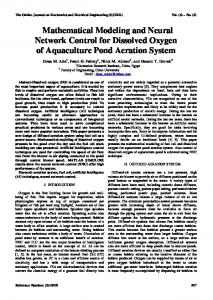
2.- The Neural Modeling Method The neural modeling method is shown in figure 1, and it can be broken down into a cycle of seven stages: from problem specification to determination of new experimental paradigms and transfer to engineering.
2.1.- Biological experimental analysis. In this stage the biological behavior (human, or animal) is defined. These aspects can be categorized in a general way as perceptual, cognitive and motion tasks. The observation of and search for invariant characteristics of the behavior under study characterize this stage. These invariant characteristics or features define the biological principles that we want to model. The results of psychophysical experiments are analyzed to determine hypotheses about the operation of certain systems of the brain. For example, in ∗
Instituto de las Tecnologías de la Producción Escuela Técnica Superior de Ingenieros Industriales Paseo del Cauce s/n 47011 Valladolid, Spain Tel: +34 983 423545 Fax: +34 983 423358 Email:
[email protected]
the area of motion aspects of the coordination of movement in the human can be studied such as: form of trajectories, synchronization of the joints, duration of movements [1,2]. In the area of perception, the effect of the structure of the visual stimuli and their intrinsic attributes (color, size, texture, form) is studied. For example, we can cite the preservation of color perception or brightness of the images independently of the visual context. In the case of cognitive tasks, as is the case of the memory we try to analyze the capacity of the system to store information of different nature in different temporal scales (eg. Short Term Memory and Long Term Memory).
2.2- Comparison with the biology of the system under study. In this stage, an attempt is made to delimit the possible neural mechanisms that produce the behavior under study. The connectivity and topology of the brain at local, regional and system levels are studied to define the structure and operation of the systems. 1.
Biological experimental analysis
7. Model prediction and transfer to engineering
2. Comparison with the biology under study
6.- Analysis of emergent properties
3. Mathematical formulation of the model
5. Comparison with initial characteristics of
4.- Model simulation
Figure 1.- Neural modeling cycle
2.3.- Mathematical formulation of the model. Once the behavioral biology to model has been defined, it is necessary to specify a mathematical model that can produce that behavior. The proposed approach is to model the behaviors as dynamical systems through non-linear differential equations to represent either the voltage of the membrane or to define the dynamics of neurotransmitters and the learning or adaptation rules. Thus for example, Grossberg [3] has developed the shunting model based on the equation of Hodgkin-Huxley [4] that describes the behavior of the neuron membranes. The equation that describes the shunting network is: dxi = − A xi + ( B − xi ) I i − xi å I j dt j ≠i where xi represents the membrane potential or activity of neuron i, and Ii is the input signal to the neuron i. The term A xi represents the passive decay of the neuron activity i, where, in absence of excitation the activity decreases until zero to a rate of A. On the other hand, the second term represents the excitation that attempts to carry the activity level of the neuron i at a maximum saturation level. Finally, the last term represents the lateral inhibitions produced by the neighbor neurons.
2.4.- System simulation. At this point a methodology to carry out the simulation in a computer is needed. It can be used specific simulation languages or system programming languages (eg. C language) as those present the advantage of a better integration for the development of real time applications. As it is necessary to simulate nonlinear dynamical systems, it is necessary to use algorithms for numerical the resolution of differential equations (eg. Runge Kutta, Euler, etc.). Different aspects must be considered such as the integration step
and the commitment between speed and precision. For system debugging it is necessary to plot the internal system variables and to verify that they represent expected values. On some occasions it may be necessary to develop graphical interfaces that permit the system behavior to be visualized during the simulation running.
2.5.- Comparison with the initial characteristics of operation. The results of the simulation are compared with the initial characteristics of operation extracted in the first stage. We can say that a variable or a system state of the modeled system reproduces the behavior of a biological variable if the first generates a trajectory that is comparable with the biological variable (activity of the particular neuron) or behavior (e.g. position or speed of a joint). It is desirable to obtain statistical analysis of the simulated variables in order to compare averaged outputs of several simulations with real measurements. To introduce variability in the simulations, it is desirable to introduce noise in the system to be simulated, either in the input of the system or in the parameters of the model.
2.6.- Analysis of emergent properties. One of the aims of the neural modeling procedure is to discover emergent properties of the system that result from the collective behavior of the variables. Typically, these properties arise from the interconnection of different modules, which may have different temporal or spatial scales. For example, we will show in the model proposed for the reactive navigation of a mobile robot how, after the definition of a set of behaviors (stroll, avoid, wall following, etc). the robot is able to compose them and to develop more complex navigation tasks.
2.7.- Model prediction and development Another objective of the modeling cycle is to predict the response of the system to different operation conditions to those initially defined. The last objective is to transfer the biological principles and the neural mechanisms to the engineering development in order to imitate the infrastructure and the neural algorithms in tasks that are accomplished by biological systems. For example, it is possible to design a robot or manipulator after the study of the human arm movement.
3.- The Neural modeling approach to the navigation of a mobile robot. In the rest of the paper we will apply the described neural modeling methodology to the design of a neural model for the adaptive navigation of a mobile robot. One of the tasks that humans and animals have to face is to choose rapidly and correctly between the different alternative motor responses. In the case of a mobile robot it is necessary to determine how to navigate and to go to a certain destination without colliding with the obstacles in the environment with the help of the information perceived by the sensors. The organisms are able to learn by themselves without external teachers to combine sensorial information and motor responses to operate in unknown and changing environments. The study of the psychology and ethology permits us to observe that animals and humans have to learn to predict the consequences of their own actions. By learning the causality of environmental events, it becomes possible to predict future and new events. With this type of learning, also known as operant conditioning, an animal learns to exhibit more frequently a behavior that has lead to a reward, and to exhibit less frequently a behavior that has lead to Punishment [5]. This notion of reward and punishment reinforces the causal behavior and provides a useful model for the behavioral modification in robotics. The appeal of these learning models is that they do not need an external supervisor that tells the system the objective, since the evaluation of its own behavior permits the system to adjust and to improve its future response. One of the problems associated with reinforcement learning is the credit assignment problem. For example, a hungry cat placed in a cage from which it can see some food will learn to press a lever that allows it to escape the cage to reach the food. In this situation the animal cannot simply wait for things to happen, but it must generate different behaviors and learn which are effective. The main problem of modeling this type of behavior is to determine, from all the behaviors, which one produces the reward.
The proposed navigation model is based in the combination of a set of behaviors, which are activated depending on the sensorial information. The behaviors can be classified in two groups, depending on the type of response and learning: reflex and adaptive. The reflex behaviors, by analogy with live beings, are the behaviors that exist from the beginning and need not be learned. They are activated as a result of intensive stimuli (when the hand gets too close to the fire, produces a sudden pain or a panic reaction) or instinctive needs for life (a newborn does not need to learn to suck) and the performance is immediate and intuitive. As a rule, in these kinds of stimuli the fundamental factor is response time, since it is necessary to act with the maximum speed to avoid possible irreversible damage. In the case of the mobile robot, an example of instinctive behavior would be that of being faced with a collision. This behavior is active when the contact sensors perceive the pressure of an obstacle on the robot. In this situation the robot stops and moves back to be removed from the obstacle to avoid damage, since, if this situation continues, the motors could be damaged; thus, a rapid and not too complex response is necessary to reverse the situation. They have been defined as instinctive behaviors: collision, stroll and correct. • •
•
Collision: This is the situation in which the robot crashes against an obstacle, where some of the bumper sensors are activated. The robot must react with a reflexive behavior that permits the robot to be removed from the obstacle Stroll: If an obstacle is detected very close in the direction of movement, the robot stops and turns in the opposite direction to the obstacle. Correct: The robot takes a direction without varying it, until a new behavior is elicited.
The adaptive behaviors need a previous study of the process and of the correct selection of the performance commands. Furthermore, the learning and development of these behaviors is possible, based on the use of evaluation techniques. These characteristics permit the robot to adapt to changing situations through a reinforcement learning process, where the commands that permit the robot to operate in a correct way (absence of collisions, goal reaching in the shortest possible time) are primed, allowing the system to evolve toward an accurate operation. They have been defined as adaptive behaviors: avoid, wall following and goal reaching. • • •
Avoid: Upon detecting an obstacle at a moderate distance, the robot turns avoiding the obstacle and continues its travel. Wall Following: Once a wall or an obstacle is detected in a lateral of the robot, this follows the wall at a given distance. Goal Reaching: If there is no obstacle in the direction of a destination point, the robot goes towards it.
The proposed neural model shown in figure 2 is made up of several interconnected modules which, through a perception-action cycle, allows the robot to obtain the linear and angular velocities. In general terms, the operation of the model is as follows. The intermodal map receives information from the infrared sensors, ultrasonic sensors and the robot bumper. This information is processed through contrast and reinforcement mechanisms that allows us to obtain signals less exposed to noise and uncertainties. Once the information is contrasted, the information flows to the behavior module, where a behavior is elicited, and additionally to the sensorial module, where a behavioral representation of the environment is obtained. The sensorial map is connected to the velocity vector through adaptive connections and defines the appropriate linear angular velocities for that situation and the active behavior. The VITE module [6] transforms this speed to avoid sharp jumps or discontinuities, and thus to obtain a soft speeds profile. The learning is accomplished in three modules. In the behaviors map, where the robot learns to select a behavior depending on sensor information. In the velocity vector, where the robot learns the velocity distribution that is appropriate for each behavior. Furthermore, an adaptive process is produced in the sensor map that allows the codification of the sensorial states that the robot detects in each behavior by means of self-organizing networks.
Intermodal
Behaviors Map
Sensorial Map Velocity Vector
Sensors
VITE
Externa l Inputs
V W ROBOT Fig. 2. General scheme of the proposed model.
The system has been modeled through two different time scale differential equations: •
Short time scale differential equations which represent fast dynamics and information is coded as the activity of neurons, that remains active for a short period of time when the excitation stops. For example the behaviors map is modeled as the following Shunting On-Center Off-Surround equation [8] :
dC i + = −γ C i + ( B − C i )( E i K i å [wij − S j ] + f (C i )) − å f (C j ) dt j j ≠i where Ci represents the activity of the behavior i, Ei characterizes the internal motivation state of the robot, Ki shows the relative importance of the ith behavior (for instance, stroll has priority with respect to avoid or wall following) and wij represents the adaptive weights of the Intermodal Map and the behavior i. Depending on the shape of the function Ci, linear, faster than linear, slower than linear or sigmoid, different dynamics are obtained. In particular, with a faster than linear function the competition means that only one behavior is active (winner takes all). •
Long time scale differential equations, which represent long term dynamics information, which prevail through time, and represent the weights learning equations. For example, reinforcement learning permits the robot to anticipate future collisions after several crashes detected by the bumper. The equation that describes this behavior is:
dw iST = −η ⋅ w iST + ( B − w iST ) P ⋅ S i dt where wi is the adaptive weight which defines the safety distance domain that the robot has to consider in order to change the direction of movement to avoid collision with an obstacle. Si is the activity of neuron i of the intermodal map that represents the proximity of an obstacle detected by the ith sensor and P is the collision signal detected by the bumper. The dynamic nature of the equations permits the association in time between the instant of the collision and the previous time, while the activity of sensor information remains active. A complete description of the equations of the model can be seen in [7].
The architecture has been simulated and the performance tested under different conditions and in different environments. Figure 3 shows several environments with different configurations of the obstacles and how the robot reaches its destination. The combination of the elementary behaviors produce an emergent complex behavior which permits the robot to reach destinations at arbitrary points in complex environments.
0
(
(
In figure 4 the evolution of the avoiding 0 behavior is shown at a stage without initial learning, and after 5000, 10000, and 20000 learning iterations. At the beginning the safety ( ( domains has not been learned and the robot crashes against walls and obstacles, but after and Figure 3. Destinations scope in complex environments. initial learning the robot starts to avoid efficiently the obstacles. The continuous learning while the robot is in operation allows the robot to adapt to the characteristics of the environment. For example, the robot develops greater angular velocities in cluttered environments than when the robot operates in spacious environments. After testing the correct operation of the neural controller in the simulation, it has been tested in a real robot Nomad. This robot is driven by a sycho-drive mechanism (one motor to drive the wheels and a second motor to steer all the wheels), and is equipped with pressure sensitive sensors to detect collisions, sonar and infrared sensors to detect and determine distance to obstacles, and a 2D laser system to obtain the profile of objects.
(a)
(c)
(b)
(d)
Figure 4. Evolution of the learning for the avoid behavior: (a) without learning, (b) after 5000 iterations, (c) after 10000 iterations, and (d) after (
(
(
(
Figure 5. Different tours of the robot in a real environment in exploration mode.
20000 iterations. Several tours developed by the Nomad in exploration mode are shown in figure 5. It can be observed that the activation of the different behaviors endows the robot with great capacity to recognize important characteristics of the environment. It is possible to recognize convex and concave corners, narrow corridors, obstacle free space, walls, persons or other mobile obstacles, etc. This capacity would make the generation of environment maps and their updating and maintenance possible.
4.- References [1] Georgopoulos, A., Kalaska, J., & Massey, J. Spatial trajectories and reaction times of aimed movements: Effects of practice, uncertainty, and change in target localization. Journal of Neurophysology, 46, 725–743, 1981.
[2] Morasso, P. Spatial control of arm movements. Experimental Brain Research, 42,223–227, 1981. [3] Grossberg, S. Contour enhancement, short term memory, and constancies in reverberating neural networks. Studies in Applied Mathematics, 52, 217–257, 1973. [4] Hodgkin, A., & Huxley, A. A quantitative description of membrane current and its application to conduction and excitation in nerve. Journal of Physiology, 117, 500–544, 1952. [5] Bullock, D., & Grossberg, S. The VITE model: A neural command circuit for generating arm and articulator trajectories. Dynamic Patterns In Complex Systems, 305–326, 1988. [6] Thorndike. Animal Intelligence, Hafner, Darien, C.T., 1981. [7] Zalama. E. Adaptive Behavior Navigation of a Mobile Robot. Technical Report TR12-99, Instituto Tecnologías de la Producción, University of Valladolid. 1999.