The noise component in model-based cluster analysis Christian Hennig1 and Pietro Coretto2 1
2
Department of Statistical Science, University College London, Gower St, London WC1E 6BT, United Kingdom
[email protected] Dipartimento di Scienze Economiche e Statistiche Universita degli Studi di Salerno 84084 Fisciano - SA - Italy
[email protected]
Abstract. The so-called noise-component has been introduced by Banfield and Raftery (1993) to improve the robustness of cluster analysis based on the normal mixture model. The idea is to add a uniform distribution over the convex hull of the data as an additional mixture component. While this yields good results in many practical applications, there are some problems with the original proposal: 1) As shown by Hennig (2004), the method is not breakdown-robust. 2) The original approach doesn’t define a proper ML estimator, and doesn’t have satisfactory asymptotic properties. We discuss two alternatives. The first one consists of replacing the uniform distribution by a fixed constant, modelling an improper uniform distribution that doesn’t depend on the data. This can be proven to be more robust, though the choice of the involved tuning constant is tricky. The second alternative is to approximate the ML-estimator of a mixture of normals with a uniform distribution more precisely than it is done by the “convex hull” approach. The approaches are compared by simulations and for a real data example.
1 Introduction Maximum Likelihood (ML)-estimation of a mixture of normal distributions is a widely used technique for cluster analysis (see, e.g., Fraley and Raftery (1998)). Banfield and Raftery (1993) introduced the term “model-based cluster analysis” for such methods. In the present paper we are concerned with an idea for improving the robustness of these estimators against outliers and points not belonging to any cluster. For the sake of simplicity, we only deal with one-dimensional data here, but the theoretical results carry over easily to multivariate models. See Section 6 for a discussion of computational issues in the multivariate case. Observations x1 , . . . , xn are modelled as i.i.d. according to the density
2
Christian Hennig and Pietro Coretto
fη (x) =
s X
πj ϕaj ,σj2 (x),
(1)
j=1
where η = (s, a1 , . . . , as , σ1 , . . . , σs , π1 , . . . , πs ) is the parameter vector, the number of components s ∈ IN may be known or Punknown, (aj , σj ) pairwise distinct, aj ∈ IR, σj > 0, πj > 0, j = 1, . . . , s, sj=1 πj = 1 and ϕa,σ2 is the density of the normal distribution with mean a and variance σ 2 . Estimators of the parameters are denoted by hats. There is a problem with the ML-estimation of η. If a ˆj = xi for some i, a mixture component j and σ ˆj → 0, the likelihood converges to infinity and the ML-estimator is not properly defined. This has to be prevented by a restriction. σj ≥ c0 > 0 ∀j for a given c0 or σi ≥ c0 > 0, i, j = 1, . . . , s, σj
(2)
ensure a well-defined ML-estimator (up to label switching of the components). In the present paper we use (2), see Hathaway (1985) for theoretical background. Having estimated the parameter vector η by ML for given s, the points can be classified by assigning them to the mixture component for which the estimated a posteriori probability pij that xi has been generated by the mixture component j is maximized: cl(xi ) = arg max pij , j
π ˆj ϕaˆj ,ˆσj (xi ) . ˆk ϕaˆk ,ˆσk (xi ) k=1 π
pij = Ps
(3)
In cluster analysis, the mixture components are interpreted as clusters, though this is somewhat controversial, because mixtures of more than one not well separated normal distributions may be unimodal and could look quite homogeneous. It is possible to estimate the number of mixture components s by the Bayesian Information Criterion BIC (Schwarz (1978)), which is done for example by the add-on package “mclust” (Fraley and Raftery (1998)) for the statistical software systems R and SPLUS. In the present paper we don’t treat the estimation of s. Note that robustness for fixed s is important as well if s is estimated, because the higher s, the more problematic the computation of the ML-estimator, and therefore it is important to have good robust solutions for small s. Figure 1 illustrates the behaviour of the ML-estimator for normal mixtures in the presence of outliers. The addition of one extreme point to a data set generated from a normal mixture with three mixture components has the effect that the ML estimator joins two of the original components and fits the outlier alone by the third component. Note that the solution depends on
0.05
0.10
0.15
0.20
0.25
0.30
3
0.00
0.00
0.05
0.10
0.15
0.20
0.25
0.30
The noise component in model-based cluster analysis
0
5
10
−5
0
5
10
15
20
Fig. 1. Left side: artificial data generated from a mixture of three normals with normal mixture ML-fit. Right side: same data with one outlier added at 22 and ML-fit with c0 = 0.01.
the choice of c0 in (2), because the mixture component to fix the outlier is estimated to have minimum possible variance. Various approaches to deal with outliers are suggested in the literature about mixture models (note that all of the methods introduced below work for the data in Figure 1 in the sense that the outlier on the right side doesn’t affect the classification of the points on the left side, provided that not too unreasonable tuning constants are chosen where needed). Banfield and Raftery (1993) suggested to add a uniform distribution over the convex hull (i.e., the range for one-dimensional data) to the normal mixture: fη (x) =
s X j=1
Ps
πj ϕaj ,σj2 (x) + π0
1(x ∈ [xmin , xmax ]) , xmax − xmin
(4)
j=0 πj = 1, π0 ≥ 0, xmax and xmin denote the maximum and minimum of the data. The uniform component is called the “noise component”. The parameters πj , aj and σj can again be estimated by ML (“BR-noise” in the following”). As an alternative, McLachlan and Peel (2000) suggest to replace the normal densities in (1) by the location/scale family defined by tν -distributions (ν could be fixed or estimated). Other families of distributions yielding more robust ML-estimators than the normal could be chosen as well, such as Huber’s least favourable distributions as suggested for mixtures by Campbell (1984). A further idea is to optimize the log-likelihood of (1) for a trimmed set of points, as has already been proposed for the k-means clustering criterion (Cuesta-Albertos, Gordaliza and Matran (1997)). Conceptually, the noise component approach is very appealing. t-mixtures formally assign all outliers to mixture components modelling clusters. This is
4
Christian Hennig and Pietro Coretto
0.06 0.04 0.00
0.02
Density
0.04 0.00
0.02
Density
0.06
not appropriate in most situations from a subject-matter perspective, because the idea of an outlier is that it is essentially different from the main bulk of the data, which in the mixture setup means that it doesn’t belong to any cluster. McLachlan and Peel (2000) are aware of this and suggest to classify points in the tail areas of the t-distributions as not belonging to the clusters, but mathematically the outliers are still treated as generated by the mixture components modelling the clusters.
0
10
20
30
40
50
60
70
0
10
20
Votes in percent
30
40
50
60
70
Votes in percent
0.06 0.04 0.00
0.02
Density
0.04 0.00
0.02
Density
0.06
Fig. 2. Left side: votes for the republican candidate in the 50 states of the USA 1968. Right side: fit by mixture of two (thick line) and three (thin line) normals. The symbols indicate the classification by two normals.
0
10
20
30
40
Votes in percent
50
60
70
0
10
20
30
40
50
60
70
Votes in percent
Fig. 3. Left side: votes data fitted by a mixture of two t3 -distributions. Right side: fit by mixture of two normals and BR-noise. The symbols indicate the classifications.
The noise component in model-based cluster analysis
5
On the other hand, the trimming approach makes a crisp distinction between trimmed outliers and “normal” non-outliers, while in reality it is often unclear whether points on the borderline of clusters should be classified as outliers or members of the clusters. The smoother mixture approach via estimated a posteriori probabilities by analogy to (3) applied to (4) seems to be more appropriate in such situations, while still implying a conceptual distiction between normal clusters and the outlier generating uniform distribution. As an illustration, consider the dataset shown on the left side of Figure 2 giving the votes in percent for the republican candidate in the 1968 election in the USA (taken from the add-on package “cluster” for R). The main bulk of the data can be roughly separated into two normally looking clusters and there are several states on the left that look atypical. However, it is not so clear where the main bulk ends and states begin to be “outlying”, neither is it clear whether the state with the best result for the republican candidate should be considered an outlier. On the right side you see ML-fits by normal mixtures. For s = 2 (thick line), one mixture component is taken to fit just three outliers on the left, obscuring the fact that two normals would yield a much more convincing fit for the vast majority of the higher election results. The mixture of three normals (thin line) does a much better job, although it joins several points on the left as a third “cluster” that don’t have very much in common and don’t look very “normal”. The t3 -mixture ML runs into problems on this dataset. For s = 2, it yields a spurious mixture component fitting just four packed points (Figure 3, left side). According to the BIC, this solution is better than the one with s = 3, which is similar two the normal mixture with s = 3. On the right side of Figure 3 the fit with the noise component approach can be seen, which is similar to three normals in terms of point classification, but provides a useful distinction between normal “clusters” and uniform “outliers”. Another conceptual remark concerns the interpretation of the results. It makes a crucial difference whether a mixture is fitted for the sake of density estimation or for the sake of clustering. If the main interest is in cluster analysis, it is of major importance to interpret the classification and the distinction between “cluster” and “outlier” can be very useful. In such a situation the uniform distribution for the noise component is not chosen because we really believe that the outliers are uniformly distributed, but to mimic the situation that there is no prior information where outliers could be and what could be their distributional shape. The uniform distribution can then be interpreted as “informationless” in a subjective Bayesian fashion. However, if the main interest is density estimation, it is much more important to come up with an estimator with a reasonable shape of the density. The discontinuities of the uniform may then be judged as unsatisfactory and a mixture of three or even four normals may be preferred. In the present paper we focus on the cluster analytical interpretation. In Section 2, some theoretical shortcomings of the original noise component approach are highlighted and two alternatives are proposed, namely replacing
6
Christian Hennig and Pietro Coretto
the uniform distribution over the range of the data by am improper uniform distribution and estimating the range of the uniform component by ML. In Section 3, theoretical properties of the different noise component approaches are discussed. In Section 4, the computation of the estimators using the EM-algorithm is treated and some simulation results are given in Section 5. The paper is concluded in Section 6. Note that the theory and simulations in this paper are an overview of more detailed results in Pietro Coretto’s forthcoming PhD thesis. Proofs and detailed simulation results will be published elsewhere.
2 Two variations on the noise component 2.1 The improper noise component Hennig (2004) has derived a robustness theory for mixture estimators based on the finite sample addition breakdown point by Donoho and Huber (1983). This breakdown point is defined, in general, as the smallest proportion of points that has to be added to a dataset in order to make the estimation arbitrarily bad, which is usually defined by at least one estimated parameter converging to infinity under a sequence of a fixed number of added points. In the mixture setup, Hennig (2004) defined breakdown as aj → ∞, σj2 → ∞, or πj → 0 for at least one of j = 1, . . . , s. Under (4), the uniform component is not regarded as interesting on its own, but as a helpful device, and its parameters are not included in the breakdown point definition. However, Hennig (2004) showed that for fixed s the breakdown point not only for the normal mixtureML, but also for the t-mixture-ML and BR-noise is the smallest possible; all these methods can be driven to breakdown by adding a single data point. Note, however, that a point has to be a very extreme outlier for the noise component and t-mixtures to cause trouble, while it’s much easier to drive conventional normal mxtures to breakdown. The main robustness problem with the noise component is that the range of the uniform distribution is determined by the most extreme points, and therefore it depends strongly on where the outliers are. A better breakdown behaviour (under some conditions on the dataset, i.e., the components have to be well separated in some sense) has been shown by Hennig (2004) for a variant in which the noise component is replaced by an improper uniform density k over the whole real line: fη (x) =
s X
πj ϕaj ,σj2 (x) + π0 k.
(5)
j=1
k has to be chosen in advance, and the other parameters can then be fitted by “pseudo ML” (“pseudo” because (5) does not define a proper density and therefore not a proper likelihood). There are several possibilities to determine k:
The noise component in model-based cluster analysis
•
• •
7
a priori by subject matter considerations, deciding about the maximum density value for which points cannot be considered anymore to lie in a “cluster”, exploratory, by trying several values and choosing the one yielding the most convincing solution, estimating k from the data. This is a difficult task, because k is not defined by a proper probability model. Interpreting the improper noise as a technical device to fit a good normal mixture for most points, we propose the following technique: 1. Fit (5) for several values of k. 2. For every k, perform classification according to (3) and remove all points classified as noise. 3. Fit a simple normal mixture on the remaining (non-noise) points. 4. Choose the k that minimizes the Kolmogorow distance between the empirical distribution of the non-noise points and the fit in step 3. Note that this only works if all candidate values for k are small enough that a certain minimum portion of the data points (50%, say) is classifed as non-noise. From a statistical point of view, estimating k is certainly most attractive, but theoretically it is difficult to analyze. Particularly, it requires a new robustness theory because the results of Hennig (2004) assume that k is chosen independently of the data. The result for the voting data is shown on the left side of Figure 4. k is lower than for BR-noise, so that the “borderline points” contribute more to the estimation of the normal mixture. The classification is the same. More improvement could be seen if there was a further much more extreme outlier in the dataset, for example a negative number caused by a typo. This would affect the range of the data strongly, but the improper noise approach would still yield the same classification. Some alternative techniques to estimate k are discussed in Coretto and Hennig (2007).
2.2 Maximum likelihood with uniform A further problem of BR-noise is that the model (4) is data dependent, and its ML estimator is not ML for any data independent model, particularly not for the following one: fη (x) =
s X
πj ϕaj ,σj2 (x) + π0 ub1 ,b2 (x),
(6)
j=1
where ub1 ,b2 is the density of a uniform distribution on the interval [b1 , b2 ]. This may come as a surprise, because the range of the data is ML for a single uniform distribution, but if it is mixed with some normals, the range of the data is not ML anymore for b1 and b2 , because fη is nonzero outside [b1 , b2 ]. For example, BR-noise doesn’t deliver the ML solution for the voting
8
Christian Hennig and Pietro Coretto
0.06 0.04 0.00
0.02
Density
0.04 0.00
0.02
Density
0.06
data, which is shown on the right side of Figure 4. In order to prevent the likelihood from converging to infinity for b2 − b1 → 0, the restriction (2) has 2 −b1 to be extended to σ0 = b√ , the standard deviation of the uniform. 12
0
10
20
30
40
Votes in percent
50
60
70
0
10
20
30
40
50
60
70
Votes in percent
Fig. 4. Left side: votes data fitted by (5) with s = 2 and estimated k. Right side: fit by ML for (6), s = 2. The symbols indicate the classifications.
Taking the ML-estimator for (6) is an obvious alternative (“ML-uniform”). For the voting data the ML solution to fit the uniform component only on the left side seems reasonable. The largest election result is now assigned to one of the normal clusters, to the center of which it is much closer than the outliers on the left to the other normal cluster.
3 Some theory Here is a very rough overview on some theoretical results which will be published elsewhere in detail: Identifiability. All parameters in model (6) are identifiable. This is not surprising because the uniform can be located by the discontinuities in the density (defined as the derivative of the cdf), and mixtures of normals are identifiable. The result involves a new definition of identifiability for mixtures of different families of distributions, see Coretto and Hennig (2006). Asymptotics. Note that the results below concern parameters, but asymptotic results concerning classification can be derived in a straightforward way from the asymptotic behaviour of the parameter estimators. BR-noise. n → ∞ ⇒ 1/(xmax − xmin ) → 0 whenever s > 0. This means that asymptotically the uniform density is estimated to be zero (no points are classified as noise), even if the true underlying model is (6) including a uniform.
The noise component in model-based cluster analysis
9
ML-uniform. This is consistent for model (6) under (2) including the standard deviation of the uniform. However, at least the estimation of b1 and b2 is not asymptotically normal because the uniform distribution doesn’t fulfill the conditions for asymptotic normality of MLestimators. Improper noise. Unfortunately, even if the density value of the uniform distribution in (6) is known to be k, the improper noise approach doesn’t deliver a consistent estimate for the normal parameters in (6). Its asymptotics concerning the canonical parameters estimated by (5), i.e., the value of its “population version”, is currently investigated. Robustness. Unfortunately, ML-uniform is not robust according to the breakdown definition given by Hennig (2004). It can be driven to breakdown by two extreme points in the same way BR-noise can be driven to breakdown by one extreme point, because if two outliers are added on both sides of the original dataset, BR-noise becomes ML for (6). The improper noise approach with estimated k is robust against the addition of extreme outliers under a sensible initial range of k. Its precise robustness properties still have to be investigated.
4 The EM-algorithm Nowadays, the ML-estimator for mixtures is often computed by the EMalgorithm, which is shown in various settings to increase the likelihood in every iteration, see Redner and Walker (1984). The principle is as follows: Start with some initial parameter values which may be obtained by an initial partition of the data. Then iterate the E-step and the M-step until convergence. E-step: compute the posterior probabilities (3), their analogues for the model under study, respectively, given the current parameter values. M-step: compute component-wise ML-estimators for the parameters from weighted data, where the weights are given by the E-step. For given k, the improper noise estimator can be computed precisely in the same way. The proof in Redner and Walker (1984) carries over even though the estimator is only pseudo-ML, because given the data, the improper noise component can be replaced by a proper uniform distribution over some set containing all data points with a density value of k. For ML-uniform it has to be taken into account that the ML-estimator for a single uniform distribution is always the range of the data. This means for the EM-algorithm that whatever initial interval I is chosen for [b1 , b2 ], the uniform mixture component is estimated as the uniform over the range of the data contained in I in the M-step. Particularly, if I = [xmin , xmax ], the EMestimator yields Banfield and Raftery’s noise component as ML-estimator, which is indeed a local optimum of the likelihood in this sense. Therefore,
10
Christian Hennig and Pietro Coretto
unfortunately, the EM-algorithm is not informative about the parameters of the uniform. A reasonable approximation of ML-uniform can only be obtained by starting the EM-algorithm several times, either initializing the uniform by all pairs of data points, or, if this is computationally not feasible, by choosing an initial grid of data points from which all pairs of points are used. This could be for example xmin , xmax , and all empirical 0.1q-quantiles for q = 1, . . . , 9, or the range of the data could be partitioned into a number of equally long intervals and the data points closest to the interval borders could be chosen. The solution maximizing the likelihood can then be taken.
5 Simulations Simulations have been carried out to compare the two new proposals MLuniform and improper noise with BR-noise and ML for tν -mixtures. The latter has been carried out with estimated degrees of freedom ν and classification of points as “outliers/noise” in the tail areas of the estimated t-components, according to Chapter 7 of McLachlan and Peel (2000). The ML-uniform has been computed based on a grid of points as explained in Section 4. Data sets have been generated with n = 50, n = 200 and n = 500, and several statistics have been recorded. The precise simulation results will be published elsewhere. In the present paper we focus on the average misclassification percentages for the datasets with n = 200. Data have been simulated from four different parameter choices of the model (6), which are illustrated in Figure 5. For every model, 70 repetitions have been run. Table 1. Average misclassification percentages for n = 200 Model/method Two outliers Wide noise Noise on one side Noise in between
BR-noise
t-mixture
improper noise
ML-uniform
2.7 8.0 10.6 8.8
7.3 9.6 8.3 8.7
3.9 8.4 3.6 5.5
3.3 9.3 5.3 7.3
The misclassification results are given in Table 1. BR-noise yielded the best performance for the “wide noise” model. This is not surprising, because in this model it’s very likely that the most extreme points on both sides are generated by the uniform. With two extreme outliers on one side, it was also optimal. However, it performed much worse in the two models that generated 10% noise at particular places (“noise on one side” and “noise in between”). The improper noise approach generally performed very well, almost always better than uniform-ML (which was the best method for two of the models
The noise component in model-based cluster analysis Wide noise
0.10
Density
0.00
0.05
0.10 0.00
0.05
Density
0.15
0.15
Two outliers
11
0
5
10
15
20
25
0
5
10
15
20
x
x
Noise on one side
Noise in between
0.06
Density
0.02
0.04
0.06 0.04
0.00
0.00
0.02
Density
0.08
0.08
0.10
0.10
−5
−5
0
5
10
15
x
20
25
−5
0
5
10
15
20
25
x
Fig. 5. Simulated models. Note that for the model “2 outliers” the number of points drawn from the uniform component has been fixed to 2.
for n = 500). The t-mixtures-ML didn’t perform very well, but this is at least partly due to the fact that all simulated models were of the “normal mixture plus uniform”-type. We will also carry out simulations from t-mixtures in the future.
6 Conclusion To deal with noise and outliers in cluster analysis, two new methods have been proposed, which are variants of Banfield and Raftery’s (1993) noise component, namely the use of an improper density to model the noise and an MLestimator for a mixture model including a uniform component. Both methods have some theoretical advantages over BR-noise. Simulations showed a good performance particularly for the improper noise component with estimated
12
Christian Hennig and Pietro Coretto
density value. We find the principle to model outliers and noise by an additional (proper or improper) uniform component appealing, particularly for cluster analysis applications. It allows a smooth classification of points as “noise” or as belonging to a cluster. Of course it is desirable to apply the ideas to multivariate data as well. This is possible in a straightforward way for the improper noise approach where k is fixed in advance by subject matter considerations. Our proposal to estimate k may work as well for moderate dimensionality, but this is still under investigation. The ML-uniform approach is problematic in the multivariate setup because of the large number of potentially reasonable support sets for the uniform distribution. In principle it could be applied by assuming the support of the uniform component as rectangular and parallel to the coordinate axes defined by the variables in the data. The ML solution could then be approximated by the best of several hyperrectangles defined by pairs of data points. It remains to see whether this leads to useful clusterings.
References BANFIELD, J. D. and RAFTERY, A. E. (1993): Model-Based Gaussian and NonGaussian Clustering. Biometrics, 49, 803–821. CAMPBELL, N. A. (1984): Mixture models and atypical values. Mathematical Geology, 16, 465–477. CORETTO P. and HENNIG C. (2006): Identifiability for mixtures of distributions from a location-scale family with uniforms. DISES Working Papers No. 3.186, University of Salerno. CORETTO P. and HENNIG C. (2007): Choice of the improper density in robust improper ML for finite normal mixtures. Submitted. CUESTA-ALBERTOS, J. A., GORDALIZA, A. and MATRAN, C. (1997): Trimmed k-means: An Attempt to Robustify Quantizers. Annals of Statistics, 25, 553– 576. DONOHO, D. L. and HUBER, P. J. (1983): The notion of breakdown point. In P. J. Bickel, K. Doksum, and J. L. Hodges jr. (Eds.): A Festschrift for Erich L. Lehmann, Wadsworth, Belmont, CA, 157–184. FRALEY, C. and RAFTERY, A. E. (1998): How Many Clusters? Which Clustering Method? Answers Via Model Based Cluster Analysis. Computer Journal, 41, 578–588. HATHAWAY, R. J. (1985): A constrained formulation of maximum-likelihood estimates for normal mixture distributions. Annals of Statistics, 13, 795–800. HENNIG, C. (2004): Breakdown points for maximum likelihood-estimators of location-scale mixtures. Annals of Statistics, 32, 1313–1340. MCLACHLAN, G. J. and PEEL, D. (2000): Finite Mixture Models, Wiley, New York. REDNER, R. A. and WALKER, H. F. (1984): Mixture densities, maximum likelihood and the EM algorithm, SIAM Review, 26, 195–239. SCHWARZ, G. (1978): Estimating the dimension of a model, Annals of Statistics, 6, 461–464.
The noise component in model-based cluster analysis
13