the top-100, say, records together and returning them simultaneously, the Onion .... we present the procedures of creating and maintaining the ..... Figure 4: An illustration of retrieving and evaluating layers from the outmost inwards x1 x2 x1 x2.
The Onion T echnique: Indexing for Linear Optimization Queries Yuan-Chi Chang, Lawrence Bergman, Vittorio Castelli, Chung-Sheng Li, Ming-Ling Lo, and John R. Smith
Data Management, IBM T. J. W atson Research Center, P. O. Box, 704, Yorktown Heights, NY 10598
Abstract
quadratic, lognormal) are given ahead of the query but short of the exact model parameters, which are issued at run time. Under such circumstances, the indexing structure must take advantage of features of the given model type to avoid expensive linear scan. We began our research at the commonly used linear model, in which the sum of linearly weighted attribute values is calculated as the ranking criterion. We assume weights assigned to those attributes are unknown at the time when the index is constructed. Model-based optimization queries play an important role in information retrieval and analysis, because limiting the number of query results e�ectively summarizes the most relevant and crucial information through representative cases. In many knowledge domains, linear models are widely used for their simple mathematical properties. Depending on application scenarios, weights of the linear criterion may be known in advance, in which cases results may be pre-ranked for future queries. In other cases, weights are dynamic and thus may not be feasible to pre-compute all possible combinations. The indexing structure proposed in this paper mainly addresses the dynamic scenario. A prominent example of a linear optimization query is college ranking. Each year US News and World Report conducts studies of college education and ranks school performance by a linear weighting of quality factors such as academic reputation, faculty resources, retention rate, and so on. One such sorted table for the 1998 college ranking is shown in Figure 1. Similar examples may be found in news media and scienti c studies like ranking of the most costly cities and ranking of areas with densely populated Lyme disease vectors [6]. While the above college ranking example is based on static weights determined by magazine editors, weights can be dynamically adjusted through a web interface, which allows perspective students to generate their own ranking. If the top-N query were implemented as a SQL query like the select statement below, the whole college database would be scanned linearly. Linear scan is necessary for the full ranking. However, if only top-ten ranked schools are asked for, the fully ranked approach is undesirable. In several scienti c data retrieval scenarios we investigated, the cardinality of the database is on the order of hundreds of millions of records. Pre-processing the data to speed up run time performance becomes necessary because of its large
This paper describes the Onion technique, a special indexing structure for linear optimization queries. Linear optimization queries ask for top-N records subject to the maximization or minimization of linearly weighted sum of record attribute values. Such query appears in many applications employing linear models and is an e�ective way to summarize representative cases, such as the top-50 ranked colleges. The Onion indexing is based on a geometric property of convex hull, which guarantees that the optimal value can always be found at one or more of its vertices. The Onion indexing makes use of this property to construct convex hulls in layers with outer layers enclosing inner layers geometrically. A data record is indexed by its layer number or equivalently its depth in the layered convex hull. Queries with linear weightings issued at run time are evaluated from the outmost layer inwards. We show experimentally that the Onion indexing achieves orders of magnitude speedup against sequential linear scan when N is small compared to the cardinality of the set. The Onion technique also enables progressive retrieval, which processes and returns ranked results in a progressive manner. Furthermore, the proposed indexing can be extended into a hierarchical organization of data to accommodate both global and local queries.
Keywords: database indexing, linear optimization
1
Introduction
Linear optimization queries return database records whose linearly weighted sums of numerical attributes are ranked top-N maximally or minimally in the database. In recent years, top-N queries are often referred in the context of nearest neighbor (NN) search. The research problem we addressed and reported in this paper di�ers from NN search. We named it top-N model-based query for distinction. In top-N model-based queries, the types of models (e.g. linear, Permission to make digital or hard copies of part or all of this work or personal or classroom use is granted without fee provided that copies are not made or distributed for profit or commercial advantage and that copies bear this notice and the full citation on the first page. To copy otherwise, to republish, to post on servers, or to redistribute to lists, requires prior specific permission and/or a fee. MOD 2000, Dallas, T X USA © ACM 2000 1-58113-218-2/00/05 . . .$5.00
391
Figure 1: Linearly weighted rankings such as the college survey shown from US News and World Report(c) are widely applied as a way of information summarization volume.
occasions where short response time is desired. Although the Onion technique performs well on linear model-based queries with queries against the whole indexed set, it is much less e�ective to process queries with additional constraints to con ne the search space. The additional constraints may be as simple as bounded ranges on one or more numerical attributes or selected categorical attributes. For example, one used the Onion technique to index one million records but extra constraints from a query con ne the search to one thousand records. As a result, topN records from the one-million index may not satisfy the additional constraints at all. Using the Onion technique, the query processor will then expand the search to top-M, with M greater than N . The local versus global query dilemma is not unique to the Onion technique but applies to most nearest-neighbor indexing as well. We thus extend the Onion technique to address the local vs. global query dilemma by a hierarchical index. The hierarchy may be constructed by observing local queries to determine how to partition spatial data set or categorical attribute values. We call each partition a cluster and local queries are directed to the cluster level. Each cluster is still indexed by the aforementioned layered convex hull to achieve high performance. To keep the overhead in storage space small, the hierarchy only takes the outmost layer of each cluster to form a new convex hull at the upper level to address global queries. An alternative which doubles the storage space requirement is to construct this new convex hull with all the records from all the clusters, which we believe is a less scalable solution. The rest of the paper is organized as follows. In Section 2, we gave an overview of related work that may be used to process linear optimization queries. To the best of our knowledge, the Onion technique is the rst special indexing structure for top-N linear model-based queries. Therefore, we do not really have a reference
SELECT COLLEGE, 0.4*REPUTATION+0.3*RESOURCE+... +0.3*SELECTIVITY AS SCORE FROM COLLEGE DATABASE ORDER BY SCORE DESC
Recognizing the need of e�cient processing of top-N linear model-based queries, we propose the Onion technique as a special indexing for such queries. The Onion indexing is based on a geometric property of convex hull, which guarantees that the optimal value of a linearly weighted sum can always be found at one or more of its vertices. A convex hull is the boundary of the smallest convex region of a group of points in space. The subset of points on the boundary are the vertices. The basic idea of the Onion technique is to extend this property to construct convex hulls in layers, with outer layers enclosing inner layers geometrically. Records, along with the ID and attribute values, are indexed and grouped on disk les by the layers to which they belong. When a new query is issued with weighted numbers of record attributes, the query processing always starts from the outmost layer and evaluates records progressively inwards, much like peeling o� an onion. We show experimentally that the Onion technique achieves orders of magnitude speedup against linear scan when N is small compared to the cardinality of the set. The indexing structure has almost no overhead since we group records by their layer number and store them sequentially on disk. Furthermore, the Onion technique enables progressive retrieval which promises results returned earlier are always better than results returned later. Instead of packing the top-100, say, records together and returning them simultaneously, the Onion query processing can return the rst and best 50, while it continue on to locate the next best 50. Since the processing sequence guarantees the accuracy of ordered retrievals, this technique is most suitable to
392
point for comparison. Section 3 details the procedures of constructing and maintaining Onion indices as well as the query processing algorithm. Section 4 discusses how to build a hierarchical index, which addresses the issues of local and global queries. Section 5 presents our experimental evaluations with regard to the impact of dimension, distribution, and query size on the performance of the Onion. We conclude the paper by summarizing its bene ts and weaknesses.
2
x2
x1
Related Work
The task of nding top-N records may be posed with the maximization or minimization criterion. Since queries asking for minimal values can be conveniently turned into maximization queries by simply switching the signs of weights (coe�cients), in the rest of the paper we assume maximization queries are issued. The top-N linear modelbased query problem we wanted to solve can be written as follows. Given a set of records with m numerical attributes, nd the top N that maximizes the following linear equation. max fa � xi + a2 � xi2 + : : : + am,1 � xim,1 + am � xim g topN 1 1 (1) where (xi1 ,xi2,. . . ,xim,1 ,xim ) is the attribute value vector of the ith record and (a1 ,a2 ,.. . , am,1 ,am ) is the weighting vector. One or more of ai 's may be set to zero. When all but one dimensions are degenerated, the problem may be solved by sorting the records along the dimension with nonzero weight. One area closely related to our problem is the discipline of linear programming. In earlier works, however, linear optimization queries were referred as the problem of nding a single point or hyperplane in space which optimizes the linear criterion [7]. The search region is constrained to the intersection of half spaces speci ed by a set of linear inequalities. The processing of such a query is equivalent to solving a linear programming problem, which can be approached by techniques such as the simplex method and the ellipsoid method. Later discoveries in randomized algorithms suggested possible ways to reduce expected query response time. Seidel reported the expected time is proportional to the number of half-space constraints [13]. Matousek reported a data structure that is based on a simplicial partition tree, which is pruned by parametric search to narrow the search space [11]. Chan applied the same data structure with randomized algorithms used in tree pruning [4] to further reduce expected query processing. While linear programming sets the cornerstone of our proposed Onion technique, none of the above works, however, suggested direct extensions to answer top-N linear optimization queries. Besides the linear programming approach, it is also possible to apply linear constraint queries to spatial data indexing and then post-process the outputs. Instead of seeking for the top-N records directly, the query is processed by retrieving all the records that are greater than some threshold. Retrieved records are then evaluated and sorted to nd the top-N answers. Most studies in linear constraint queries apply spatial data structures such as Rtree and k-d-B tree. Algorithms are developed to prune the
Figure 2: Based on Fagin's algorithm [8], records falling in shaded area are retrieved to nd the maximum of x1 + x2 spatial partition tree to improve response speed. Recent publications can be found in [10]. The main di�culty of taking this two-step approach (thresholding and sorting) lies in determining the threshold which bounds the search space, especially when the spatial distribution of data is hard to estimate. A poorly chosen threshold may lead to too many or too few returns. It is also impossible to perform progressive retrieval, which allows records to be returned successively in ranking order. Another important related work is an algorithm proposed by Fagin for processing fuzzy joins [8]. He showed the applicability of the algorithm to any \upward closed" functions, which include linear weighted sum of record attributes. The algorithm was originally proposed for processing fuzzy join of multi-attribute multimedia objects in the IBM Garlic project. The query is to nd objects with maximal fuzzy combinations of attributes measured in similarity (e.g. color, shape, texture). One important distinction between Fagin's and other aforementioned works is that Fagin's algorithm does not exploit attribute correlation. Each attribute is treated independently. While this property is applicable in similarity search where attribute correlation depends on query examples, it penalizes query performance of linear optimization. An example of showing such ine�ciency is illustrated in Figure 2, where all records have two attributes, x1 and x2 . The records are distributed in a circle shown in the gure. When an optimization query is issued to nd the maximum (top-1) of the sum of the two attributes with equal weights, records falling in the shaded area marked in the circle will be retrieved and evaluated, according to the algorithm [8]. This example can be solved more ef ciently through the Onion technique. We believe while Fagin's algorithm is most applicable for applications where pre-processing is not allowed, one should take advantage of pre-processing where possible to exploit attribute correlations.
3
The Onion Technique
The basic idea of the Onion technique is to partition the collection of d-dimensional data points, which correspond to records with d numerical attributes, into sets that are optimally linearly ordered.
393
De nition 1 Optimally Linearly Ordered Sets: A collection of sets fS1 ; S2 ; : : : ; Sn g are optimally linearly
layer and number them geometrically from outside inwards starting at one. The set of layers fL1 ; L2 ; : : : ; Lm g are optimally linearly ordered. These layers constitute the index of the Onion technique. In the following subsections, we present the procedures of creating and maintaining the Onion indexing as well as the query processing steps.
ordered i� given any d-dimensional vector a,
9x 2 Si s:t:
8y 2 Si+j and j > 0; at x > at y
where at x represents the inner product of the two vectors. By this de nition, sets with lower indices always have one or more vectors whose linearly weighted sums are strictly greater than sets with higher indices. Optimally linearly ordered sets only require the existence of a d-dim vector from set Si to have a greater linearly weighted sum than any other vector from the sets ordered after Si , e.g. Si+1 , Si+2 , etc. This property does not guarantee the sets are nonredundant, i.e. each Si has the minimal number of vectors needed. Nevertheless, one can see any partition that generates optimally linearly ordered sets provides a valid indexing structure which prunes the search space of linear optimization queries. It is not di�cult to for a top-N linear model-based query, at most PNshowjS that, j records have to be evaluated. jSi j is the size of i i=1 set Si . Partitioning a set of data points into optimally linearly ordered sets may seem di�cult at rst sight. Fortunately, a theorem exists in the linear programming literature which indicates how one may perform the set partitioning.
3.1
Index Creation and Storage
The Onion technique partitions the input data set into layers, each of which is a set of data vectors. The relation between layers is best depicted geometrically using an example. Figure 3 illustrates a data set after the partition. In this gure, data records of two attributes x1 and x2 are represented as black dots scattered on the 2D plane. Three layers are formed and labeled from the outmost layer inwards, starting at Layer 1 assigned to the outmost layer. Each layer contains a variable number of records, which may be as little as one. The set of points in layer i are vertices of the convex hull of the union of all the layers below it, including itself. The Onion index is created iteratively using the convex hull construction algorithm. The procedure is described below in pseudocode. The procedure of index creation Input: the set R of data records 1 k = 1; 2 while (sizeof(R) > 0)
Theorem 1 Given a set of records R mapped to a d-
3 4 5 6 7
dimensional space, and a linear maximization (minimization) criterion, the maximum (minimum) objective value is achieved at one or more vertices of the convex hull of R.
The proof of this theorem can be found in [7] and other linear programming textbooks. The convex hull of a set R of d-dimensional vectors is de ned as the boundary of the smallest convex region containing R. The subset of vectors at the convex hull are referred as vertices or extreme points. In two dimensions, the shape of a convex hull is a polygon. In higher dimensions, its shape is a polyhedron. To see how Theorem 1 may be applied to generate optimally linearly ordered sets, one may consider the extreme case in which we only partition the set R into two subsets S1 and S2 . We compute the convex hull of R and put the vertex points into set S1 and non-vertical points into set S2 . By Theorem 1, fS1 ; S2 g forms optimally linearly ordered sets. This simple partition is su�cient to prune the search space for any top-1 queries. If N is more than one, both S1 and S2 will be searched and there is no performance advantage over linear scan. Although we will not provide a proof here, it can be shown that the set S1 is nonredundant and it contains no more vectors than necessary to satisfy the optimally linearly ordered property. The non-redundancy is desirable because this enables a partition scheme to generate P the most number of subsets possible. The worst case bound Ni=1 jSi j will be smaller. The Onion technique is based on an iteration of the convex hull partitioning. The iteration continues until the last subset can not be partitioned further without violating the linearly ordered property. We name each subset a
f
construct a convex hull of set R; store records of the hull vertices in set V ; assign records in set V to layer k; R = R - V; k = k + 1;
g
At each iteration, a convex hull of a set of data records is rst constructed using algorithms such as the gift-wrapping method and the beneath-beyond method [12]. Fast convex hull construction algorithms are not discussed in this paper and left for future topics. Records appeared as convex hull vertices are assigned to the new layer and removed from the input set. Therefore the size of the input set decreases as the iterations continue. The iteration stops when the input set becomes empty. Geometrically the partitioned structure looks like an onion, with layers corresponding to peels. Inner layers, with outer layers being vertices of their convex hulls, are wrapped spatially. This onion structure is later referred as layered convex hull. We store the data points in each layer in a number of consecutive disk pages and record the pointers to the starting and ending pages. For simplicity, each set of such pages is called a at le. Similar to the assumption made in [3], attribute values and IDs of the data records are stored together in at les. It is possible to add auxiliary indexing structures to further accelerate access to the at le. This, however, is not the focus of this paper and left for future work. This storage arrangement in e�ect clusters the input records belonging to the same Onion layer close together on disks.
394
Layer 1
Layer 3
Figure 3: A three-layered convex hull in twodimensional space
Query Evaluation
Similar to index creation, the processing of a linear optimization query also starts from the outmost layer and progresses inwards. This procedure is described as follows. The procedure of evaluating a query Input: the number of top records to return N ; coe�cients of the linear criterion 1 candidate set C = ;; 2 result set O = ;; 3 k = 1; 4 while (N > 0)
f
11 12
retrieve records in layer k and put them in a set Lk ; evaluate records in Lk with the given coe�cients; select the top N records from Lk and put them in a set T ; if (k = 1) f C =T; add the record with the maximum value in C to the result set O; remove the record from C ; N = N , 1;
13
else
7 8 9 10
move the maximal record from T to O; C =C[T; N = N , 1;
22 23
This storage structure for the Onion index has almost no overhead. After the at les are created, the only information that needs to be kept in the Onion index for later query processing is the beginning and ending page locations for each layer. As our experiments demonstrated, each layer typically contains several hundred or more data points, which makes the storage overhead negligible. While the Onion index has negligible storage overhead, the computation cost at the creation time is very high. All known algorithms of constructing convex hulls have computational complexity in the order of O(N d=2 ), where N is the size of the input data set. We acknowledge that the exponential growth in complexity as the number of dimensions increases is a serious obstacle to the Onion's applicability to high dimensional data. We leave the study of this subject to future work.
6
g
21
x1
5
if (value of c > maxT ) move c from C to the result set O; N = N , 1; if (N = 0) stop and return the result set O;
18 19 20
Layer 2
3.2
maxT = max fT g; foreach c 2 C f
14 15 16 17
x2
g f
395
g
24
k = k + 1;
25
return the result set O;
g
In this procedure, we created a candidate set, which is a container for hopeful top-N records, and a result set, which stores the records made to top N . Every time new records are added to the result set, N is decremented accordingly. In the rst iteration beginning at line number 4, the candidate set is empty and this condition is treated separately. Records at Layer 1 (the outmost layer) are retrieved and evaluated. The record with the maximum value is added to the result set. The top-2 to top-N records at Layer 1 are stored in the candidate set. Starting at Layer 2, iteration steps are identical and the iteration continues until N is decremented to zero. Without loss of generality, assume the iteration proceeds to Layer k. First, records in Layer k are read from the disk and evaluated. The best N records are kept in a set T (line 7). Next, nd the maximum value, maxT , of the set T (line 14). We describe line 7 and 14 separately for clarity while they can be implemented together. Any record in in the candidate set C that has a greater value than maxT is returned as a result. Finally, return the maximum record of Layer k and merge what remains in T into the candidate set (line 22). At any point of the process, if N becomes zero, query processing stops and the result set is returned to the client. Proof of correctness: From Theorem 1 we know the optimal record value at each layer is always greater than any record value from its inner layers. However, records in the candidate set, which come from outer layers, may still be greater than the optimal value of the next layer. The FOR loop from line 15 to 21 makes sure that those which have greater values are returned rst. Since top-N records from each layer are always added to the candidate set, one would have returned all in the candidate set, should they be greater than the maximum of the current layer. Correctness of the top-N results is thus guaranteed. Example: We use the three-layered convex hull from Figure 3 as an example to illustrate the query processing procedure. As shown in Figure 4(a), records in layer-1 are marked as 1a, 1b, 1c, 1d, and 1e. The linear optimization criterion is shown as a line which moves in its orthonormal direction. In this example, we assume the objective is to
maximize the criterion and therefore, the farther away a point from the origin in the line direction, the greater its value. N is set to three. In this example, point 1a has the largest value and is returned rst. Points 1b and 1e are put into the candidate set. Next in Figure 4(b), records in layer-2 are evaluated and 2a is returned since both 1b and 1e are smaller than 2a. At this iteration, 2e is added to the candidate set. Finally, records in layer-3 are evaluated. At this iteration, 2e from the candidate set is greater than the largest value of layer-3, 3a. Therefore, 2e is returned. The disk I/O cost of the query processing is contributed by two factors: the random access to move the disk head to the beginning disk page of a layer and the sequential access of reading pages into main memory. We assume the main memory is large enough to hold all the records in a layer. If the main memory does not have su�cient space, the sequential access may be divided into several reads. Since the query processing only requires top-N records of each layer to be kept in main memory and N is usually small, multiple disk reading operations do not increase the complexity of the processing. In the following, we prove the disk I/O cost is bounded in the worst case. Theorem 2 The disk I/O cost of evaluating a top-N linear optimization P query is bounded in the worst case by N random accesses and Nk=1 jLk j=B sequential accesses, where jLk j is the number of records stored in the kth layer and B is the number of records per disk page. Proof: By Theorem 1, each layer of the Onion index is guaranteed to provide at least one \optimal" record. When a query is issued for top-N records, at most N layers need to be accessed. Since there is one random access per layer, in the worst case there would be N random I/O's. For the rest of record retrievals, there are sequential P I/O's. The cost associated with sequential I/O's is thus Nk=1 jLk j=B . 3.3
3.4
Index Maintenance
In contrast to query processing, index maintenance operations such as inserting, deleting, and updating an Onion index are fairly complex and computationally expensive. An update operation is equivalent to a deletion followed by an insertion. We thus discuss insertion and deletion in this section. Because of the expensive computation, it may be advisable in practice to perform index maintenance in batches. The algorithm to insert a new record to an already built index is described below in pseudocode. The procedure of inserting a new record to the index Input: the new record, r 1 locate layer k such that the new record is inside the convex hull of layer k , 1 and outside the hull of layer k; (this step may be done by binary search or other methods) 2 let the set S = frg; 3 while (sizeof(S ) > 0) f 4 Lk;merge = S [ Lk ; 5 construct a convex hull of Lk;merge ; 6 store the hull vertices in set Lk;new ; 7 Lk = Lk;new ; 8 S = Lk;merge , Lk ; 9 k = k + 1;
g
The key concept is that vertices of a convex hull are not a�ected by adding or deleting points inside of the hull. As illustrated in Figure 5(a), the new record represented by the white dot is inside the hull of Layer-1. Data points in Layer-1 do not change by this insertion operation. In contrast, the white dot is outside of Layer-2. Hence points stored from Layer-2 and inner layers may have to be shifted down. The rst step of processing an insertion is to locate the neighboring layers where the new record falls in between. Once they are found, the iterations start to insert the new point and relocate existing data (line 3 to 9). Inserting a new record to a layer may cause one or more points in that layer to be expelled, as illustrated in Figure 5(b). The expelled records are inserted to the next inner layer and the operations may again expel some records from the next layer. The iteration continues when no more records are expelled or it reaches the inner-most layer. Figure 5(c) depicts such an ending. Similar to the record insertion operation, record deletions do not a�ect records in outer layers. If a record in Layerk is deleted, one or more records in Layer-(k + 1) will be moved up to Layer-k. The moved records can be thought as deletions made to Layer-(k + 1), which again solicit records from the immediately inner layer. The procedure is described below in pseudocode. Because the basic concept of the deletion operation is similar to that of insertion, we believe the pseudocode is self-descriptive and do not provide further explanations. The procedure of deleting a record Input: the record to be deleted, r 1 locate layer k where r belongs to; (this step may be implemented by a binary search since r is inside of some layers and outside of other layers)
Progressive Retrieval
One important feature enabled by the Onion indexing structure is progressive retrieval. This feature is uncommon to most indexing techniques used in ranking results. We thus wish to emphasize this feature. In many other techniques, all the records in the pruned search space are evaluated before the ranked ordering can be determined. This is not necessary using the Onion technique. As we have shown in the descriptions of query processing, the Onion technique guarantees the following property. Corollary 1 Given a linear maximization (minimization) criterion and a layered convex hull constructed using the stated procedure, the maximum (minimum) objective value achieved at layer k is strictly greater (less) than the maximum (minimum) value achieved at layer k + 1. Proof: The corollary can be easily proved by Theorem 1 and the construction procedure of the Onion index. By Corollary 1, top-N results can be progressively delivered to the client since the record ranked M is always retrieved earlier than the one ranked M + m with positive m. From the user's view point, the database thus appears to be faster since the response time to get the rst record is shortened.
396
Linear Eq.
x2 1e
1a x2
1d
1e 1c
2d
1b 1d
x1
(a)
2c
x2
3b 3a 2b
1c
1e 2d
2e
1b
2e (c)
2a
x1
1d 2c
2b
1c
1b x1
(b)
Figure 4: An illustration of retrieving and evaluating layers from the outmost inwards
4
x2
x2
(a)
x1
x2
(c)
(b)
x1
x1
Figure 5: An illustration of inserting a new record into an Onion index; the white dot represents the new record 2 3 4 5 6 7 8 9
let the set S = Lk , frg; while (sizeof(S ) > 0) f Lk;merge = S [ Lk+1 ; construct a convex hull of Lk;merge ; store the hull vertices in set Lk;new ; Lk = Lk;new ; S = Lk;merge , Lk ; k = k + 1;
g
397
Hierarchical Indexing of Onions
Although the Onion technique performs well on linear model-based queries with queries against the whole indexed set, it is much less e�ective in dealing with local queries, which have additional constraints to con ne search space. The additional constraints may be as simple as bounded attribute ranges or selected categorical attributes. Using the college ranking as an example, we found an Onion index built for colleges in the whole nation does not respond well to queries such as \top-10 colleges in the northwestern region" or \top-10 colleges with tuition below $15,000". The Onion technique does not perform well for two reasons. First, an Onion index accounts for numerical attributes of data records only, not their categorical attributes. Second, range constraints on numerical attributes e�ectively restrict the search to a subset of records that may be ranked behind globally, say starting at the 200th best. An Onion index can quickly rank and order records globally but has no way to jump directly to the 200th record. The global vs. local query dilemma does not occur to the Onion technique only. Additional constraints on most proposed indexing techniques for nearest neighbor search cause similar ine�ciency. Fortunately, for the Onion technique, we have a partial solution to the dilemma. Recognizing the global vs. local query dilemma, we extend the Onion indexing into a hierarchy with popular local queries clustered at the bottom of the hierarchy. Clusters are then selectively grouped together to form new indices at the top of the hierarchy. The grouping of clusters depends on the usage distribution of local queries as well as problem domains. In the college ranking example, it may be natural to group schools into clusters based on geological locations such as northwestern and southeastern regions. A separate Onion index is constructed for each
x2
x2 L1
L1
L2
L2
x1
x1
Figure 6: A graphical illustration of two categories of data records with distinct attribute values; using hierarchical layered convex hull indexing could further improve query processing by exploiting the structural di�erences
Figure 7: The new layered convex hull constructed from Layer-1 data records of convex hulls shown in Fig. 6 the L2 criterion is given. The query processing procedure of the hierarchical indexing is described below in pseudocode. The procedure of evaluating a query in the hierarchical indexing Input: the number of top records to return N ; coe�cients of the linear criterion 1 locate the parent Onion P corresponding to the constrained search space; 2 use the single Onion processing procedure described in Section 3.2 to nd the top-N records in P ; put them in set T ; 3 locate child Onions from which the top-N records were originated from; 4 foreach (the child Onions located above) f 5 nd the top-N records from the child Onion and put them in set C ; 6 nd the top-N records from sets T and C ; 7 update T ;
cluster to facilitate local queries. For global queries against schools nationwide, one can choose to construct a separate index to include all records. This will double the storage space requirement. Our proposed solution for hierarchical indexing is to build a global index by relying on existing local indeces. To keep the overhead in the storage space to the minimum, the global index takes the outmost layer of each cluster's index to form a new Onion. If we assume the size and location of the outmost layer approximately re ect the size and location of its cluster, the new Onion will then direct the processing to clusters which are likely to answer the query. The basic idea is best illustrated in Figures 6 and 7. In Figure 6, there are two clusters of data points expressed in black and white dots. We assume data clustering is provided by query analysis methods beyond the scope of this paper. As shown in the gure, a layered convex hull is built for each cluster to facilitate e�cient local queries. The two straight lines represent two di�erent linear optimization criterion. Due to the distinct distributions of black and white points, a linear query may be processed by one cluster only. For example, a linear query shown as a line L1 is likely to be answered by the black cluster at the left. Similarly, line L2 is likely to be answered by the white cluster. The purpose of this example is to show the possibility of pruning the search space by identifying the most relevant Onions to a given query. Figure 7 plots the new Onion index built from the outmost layers of the two Onions in Figure 6. The new index has ve records from the black cluster and ve from the white cluster. From the ten records, the new Onion forms two layers. We refer the new Onion as the parent of the white and black Onion. With a small overhead of replicating Layer-1 records, this parent index serves the purpose of pruning search space. Using this parent Onion, the query processing then knows to process the black cluster rst if the L1 criterion is given and to process the white cluster rst if
g
8 return T ; Query evaluation starts at locating the parent Onion whose child Onions meet the query constraints. Then the top-N records of the parent Onion are retrieved. At this step, these records are almost always not the top-N records we wanted since they all came from the outmost layers of child Onions. However, the child Onions where they were originated hold the true top-N records. These child Onions are accessed and combined to obtain nal results. We acknowledge that there exists better procedures that do not require each selected child Onion to generate its own top-N records. These procedures will be reported separately.
5
Experimental Evaluation
We evaluated the query processing performance of Onion indexing against simple sequential scan, which we believe serves as a good reference point since there are no other techniques addressing model-based queries. We examined the performance impact by changing the spatial distribution
398
of the data, its dimensionality, and the target number, N . Our evaluations comprised both real and synthetic data sets. The real data sets came from an environmental epidemiology study. Since experimental results from both sets behave similarly and the real data sets are not freely available for veri cation, we focus our reports on the evaluation of synthetic data sets. Our synthetic data sets comprised of four test sets, each of which contains 1,000,000 data points. In the rst and second test sets, attribute values are Gaussian distributed with mean equal to zero and variance equal to one. Points in the rst set are in a 3-dimensional space while those in the second set have 4 dimensions. The third and fourth test sets have attribute values uniformly distributed between -0.5 and 0.5. They are in 3 and 4 dimensional space, respectively. Attributes are independent of each other.
Table 2: The speedup multiple measured in computational complexity; G: Gaussian distribution, U: Uniform distribution N
1 10 100 1000
3D G 13,333 1,427 280 41
4D G 3,717 492 93 18
3D U 3,584 464 98 18
4D U 775 137 32 7
Table 3: The speedup multiple measured in disk I/O cost; G: Gaussian distribution, U: Uniform distribution N
1 10 100 1000
Our rst measurement characterizes the spread of data points across layers in an Onion index. Figure 8 plots the density distributions of points in each layer. For both uniform and Gaussian distributions, the number of layers in an Onion signi cantly decreases when the dimension increases. Less data spreading implies that query processing will be less e�cient since the partition granularity of the search space decreases. In Figure 8 we also observed an Onion of Gaussian distributed data has a larger spread than one of uniformly distributed data. This is expected since the tail of the Gaussian distribution extends to in nity, while uniformly distributed data is con ned in a data cube. The rate of decay of the probability density function a�ects data spread. Distributions with slower decay rate than Gaussian, such as exponential and Gamma, will generate even more layers. We next examine the query performance by varying N from one to one thousand. Coe�cients used in the linear criterion were randomly generated. For each test set, we ran 1,000 queries and asked for top-1,000 records. Numbers reported in Table 1 and Figure 9 are averaged over the 1,000 trials. Both in the table and the gure, the number of records evaluated and the number of layers accessed are reported. From Table 1 and Figure 9, we noticed the extent of data spreads does have a signi cant e�ect on the numbers of records and layers. In both 3 and 4 dimensional data sets, an Onion of uniform distribution requires two to three times more access than an Onion of Gaussian distribution. In higher dimensions, since more points are concentrated at the rst several layers, there are less number of layers accessed overall. However, since there are more points in each layer, high dimensional indices still require more computation.
3D G 930 208 68 16
4D G 935 217 59 14
3D U 781 162 47 11
4D U 478 104 27 6
size of the set. The more points an Onion has, the better it performs. Lastly, the performance gain measured in disk I/O is evaluated. We assume there is su�cient main memory to hold records from a single layer. Since data records in a layer are stored in a at le, sequential I/O best characterizes their access cost. One random I/O is required for loading a layer into the main memory, which requires a disk seek. Attribute values are stored in double precision. We assume a three dimensional record needs 32 bytes for storage and a four dimensional one needs 40 bytes. Each disk page holds 4K bytes. We conservatively assume the cost of one random I/O is equal to 8 times the cost of a single sequential I/O. The performance of the Onion technique will further improve if the cost of random I/O is cheaper. The formula used to compute disk I/O cost is shown in Eq. 2. Figure 10 plotted the estimated I/O cost of the four test sets. We further assume there is no random I/O cost associated with sequential linear scan. This assumption favors linear scan since it is unlikely that the main memory is always large enough. The I/O cost of scanning 1,000,000 records is xed at 8,000 sequential access for the 3D data and 10,000 access for the 4D data. Performance speedups of sampled values of N are tabulated in Table 3.
6
Conclusions
We conclude this paper by summarizing the bene ts of the Onion technique and pointing out its weaknesses and future research directions. The most appealing feature of Onion is its query processing performance, as shown in the experimental evaluations. It has almost no storage overhead, which makes it a good alternative to unstructured linear storage. Furthermore, the technique enables progressive retrieval which returns the rst record to the client at very little latency. In addition, the geometric property of convex hull which the Onion technique is based upon allows one to scale, rotate, and shift the spatial structure without changing its property. This implies the applicability of the
In terms of performance gain in computation, the Onion technique performed very well, especially when N is small. Table 2 lists the speedup against sequential scan in multiples. The numbers are generated by taking values in Table 1 and compute their ratio to 1,000,000. Orders of magnitude speedup is achievable at low N . The gain can even be higher as the size of the data set increases. In our evaluation with the real data set, we found the rate of increase in the number of evaluated records is less than the rate of increase in the
399
Table 1: The average number of records evaluated and layers accessed to retrieve top-N results from 1,000,000 points N
1 10 50 100 500 1000
3D Gaussian Records Layers 75.0 1.0 695.5 4.1 2,053.7 8.0 3,566.0 11.1 13,773.0 25.0 24,308.5 35.2
4D Gaussian Records Layers 269.0 1.0 2,030.2 3.2 6,345.9 5.9 10,641.2 7.8 33,450.0 14.4 54,820.2 18.8
I=O cost = 8 � accessed layers + 1 �
3D Uniform Records Layers 279.0 1.0 2,151.0 4.0 6,342.7 8.0 10,120.6 10.8 33,173.7 23.7 54,103.80 33.0
records evaluated �
�
4000
4D Uniform Records Layers 1,289.0 1.0 7,271.3 2.9 21,791.1 5.6 30,743.4 6.9 90,837.0 13.4 132,220.4 17.1
32 if d = 3 40 if d = 4
� (2)
1.4 3D uniform 3D Gaussian 4D uniform 4D Gaussian
1.2
Percentage of total data
1
0.8
0.6
0.4
0.2
0
0
100
200
300 400 Convex hull layer number
500
600
700
Figure 8: The density distributions of data points spread across layers in the four test sets
400
4
Number of evaluated records
14
x 10
3D uniform 3D Gaussian 4D uniform 4D Gaussian
12 10 8 6 4 2 0
0
100
200
300
0
100
200
300
400
500
600
700
800
900
1000
400 500 600 700 Number of requested records, N
800
900
1000
Number of accessed layers
40
30
20
10
0
Figure 9: Numbers of evaluated records and accessed layers when N varies from one to one thousand Onion index to a much broader category of models, not just linear weighted sums. There are a few weaknesses we have identi ed in the paper. The most prominent one is the computational complexity at the index construction time. The convex hull algorithm does not scale well into high dimensions. The dimensionality curse not only increases computational complexity but also decreases the number of layers available. Less number of layers implies lower e�ciency in pruning the search space. This is the same phenomenon that plagues spatial indexing for similarity queries, which was o�ered an explanation in [2]. Another potential weakness is its compatibility to other indexing techniques. The Onion technique is really not compatible with other spatial indexing structures like R-tree and is not e�ective in processing data cube queries. As a part of our future work, we will investigate a hybrid form of indexing structures, which hopefully will answer both top-N model-based and range queries equally well. Lastly, in our current implementation, records in a layer are atly laid out on disk. Evaluating all the records in a layer will not only obtain the maximum but also the minimum, one of which is not needed. In the future, we plan to add an auxiliary structure to organize data in a layer to avoid the ine�ciency. One simple solution is to map the Onion layers to spherical shells, which is illustrated in Figure 11. Spherical shells express layered convex hulls in concentric shells, each of which contains a layer. This gure illustrates the equivalent spherical shells of a threelayer convex hull in two dimensions. The polar coordinate of a data record is computed and only its angle is used to
x2
angle
x1
Figure 11: A graphical illustration of introducing an auxiliary structure in a layer by the angle of a data vector
order the record. The radius of a record is not used in a spherical shell and thus all data records in the same layer are shown equally distant from the origin. The query processing procedure is modi ed as follows. The linear weights of the query are rst expressed in polar coordinates, say (R; �1 ; �2 ; �3 ; :::;�d,1 ). Instead of evaluating all data records in a layer, only those records are evaluated with angles in the range of (�1 +�=2; �2 +�=2; ; : : : ; �d,1 +�=2). It is not hard to see that when data records are uniformly distributed, the spherical shell representation further decreases the number of evaluated records by half.
401
1500 3D uniform 3D Gaussian 4D uniform 4D Gaussian
Estimated disk I/O cost
1000
500
0
0
100
200
300
400 500 600 700 Number of requested records, N
800
900
1000
Figure 10: Estimated disk I/O cost of the query evaluation; for linear scan, the I/O cost is xed at 8,000 sequential page access for the 3D data and 10,000 page access for the 4D data.
7
Acknowledgments
[7] G. B. Dantzig, Linear programming and extensions, Princeton University Press, Princeton, NJ, 1963. [8] R. Fagin, \Fuzzy queries in multimedia database systems, " Proceedings of the ACM Symposium on Principles of Database Systems, pp. 1-10, 1998. [9] S. C. Fang and S. Puthenpura, Linear optimization and extentions, Prentice-Hall, Inc., Englewood Cli�s, NJ, 1993. [10] J. Goldstein, R. Ramakrishnan, U. Shaft, and J. Yu, \Processing queries by linear constraints," Proceedings of the ACM Symposium on Principles of Database Systems, pp. 257-267, 1997. [11] J. Matousek and O. Schwarzkopf, \Linear optimization queries," Proceedings of the ACM Symposium on Computational Geometry, pp. 16-25, 1992. [12] F. P. Preparata and M. I. Shamos, Computational geometry: an introduction, Springer Verlag, 1991. [13] R. Seidel, \Linear programming and convex hulls made easy," Proceedings of the ACM Symposium on Computational Geometry, pp. 211-215, 1990.
This work was funded in part by NASA/CAN NCC5-305.
References
[1] P. K. Agarwal, L. Arge, J. Erickson, P. G. Franciosa, and J. S. Vitter, \E�cient searching with linear constraints," Proceedings of the ACM Symposium on Principles of Database Systems, pp. 169-177, 1998. [2] K. S. Beyer, J. Goldstein, R. Ramakrishnan, U. Shaft, \When is nearest neighbor meaningful," Proceedings of International Conference on Database Theory, pp. 217235, 1999. [3] S. Berchtold, C. Bohm, and H. P. Kriegel, \The Pyramid-technique: towards breaking the curse of dimensionality," Proceedings of the ACM Symposium on Management of Data, pp. 142-153, 1998. [4] T. M. Chan, \Fixed-dimensional linear programming queries made easy," Proceedings of the ACM Symposium on Computational Geometry, pp. 284-290, 1996. [5] Y. C. Chang, L. Bergman, J. R. Smith, and C. S. Li, \E�cient multidimensional indexing structure for linear maximization queries," Proceedings of Multimedia Storage and Archiving Systems, Boston, MA 1999. [6] A. Das, S. R. Lele, G. E. Glass, T. Shields, and J. A. Patz, \Spatial modeling of vector abundance using generalized linear mixed models: application to Lyme disease," submitted to Biometrics for publication.
402