Multimed Tools Appl (2012) 60:261–275 DOI 10.1007/s11042-010-0614-z
Dynamic optimization of queries in pivot-based indexing Svein Erik Bratsberg · Magnus Lie Hetland
Published online: 9 October 2010 © The Author(s) 2010. This article is published with open access at Springerlink.com
Abstract This paper evaluates the use of standard database indexes and query processing as a way to do metric indexing in the LAESA approach. By utilizing B-trees and R-trees as pivot-based indexes, we may use well-known optimization techniques from the database field within metric indexing and search. The novelty of this paper is that we use a cost-based approach to dynamically evaluate which and how many pivots to use in the evaluation of each query. By a series of measurements using our database prototype we are able to evaluate the performance of this approach. Compared to using all available pivots for filtering, the optimized approach gives half the response times for main memory data, but much more varied results for disk resident data. However, by use of the cost model we are able to dynamically determine when to bypass the indexes and simply perform a sequential scan of the base data. The conclusion of this evaluation is that it is beneficial to create many pivots, but to use only the most selective ones during evaluation of each query. R-trees give better performance than B-trees when utilizing all pivots, but when being able to dynamically select the best pivots, B-trees often provide better performance. Keywords Similarity search · Pivot-based indexing · Database trees · Optimized query processing 1 Introduction Similarity search is gaining interest both for structured and unstructured objects. It is also important in domains where canonical ordering of data is not possible, for S. E. Bratsberg (B) · M. L. Hetland Department of Computer and Information Science, Norwegian University of Science and Technology, 7491 Trondheim, Norway e-mail:
[email protected] M. L. Hetland e-mail:
[email protected]
262
Multimed Tools Appl (2012) 60:261–275
instance multidimensional vector spaces or general metric spaces. The domains we will investigate contain either large vector spaces, or prohibitively expensive exact distance calculations, making a full scan to answer similarity queries costly. A query is typically formalized as a sample object, and the query is evaluated against a database of objects by issuing comparison of similarity. There are many applications of metric indexing and search. These range from entertainment and multimedia to science and medicine, or applications that require efficient query-by-example, but where traditional spatial access methods cannot be used. Beyond direct search, similarity retrieval can be used internally in a wide spectrum of systems, such as nearest neighbor classification, compressed video streaming and multiobjective optimization [12]. Our motivation is to exploit database internals such as index structures and query processing as a means to solve similarity queries. We have chosen to work with the pivot-based LAESA approach to metric indexing and search [17]. There are several existing works that have done similar research [14, 15, 23], and we build on these by exploiting more database internal techniques, having direct access to indexes, buffers and algebraic query processing capabilities. Our approach has been to exploit B+-trees and R*-trees and to use parallel hash joins in between sequential range scans of these ordered indexes. Our conclusion is that R*-trees seem to be best, especially at querying time. The use of these indexes is dependent on the query, i.e., the larger the range limit of the query, the less useful the indexes become. Furthermore, the query will be most efficiently processed using statistics on how many and which indexes to use. This is well known in database systems since the System-R days [21]. We have exploited this idea and created statistics for each access path, both for scans, B+-trees and R*-trees. Before we evaluate a query we calculate the estimated cost of executing the query using different access paths. This allows us to use the most optimal query execution strategy based on a dynamic optimization for each query. When sequential scans are estimated to be cheapest, this will be chosen to evaluate the query. The main contribution of this paper is the application of statistics to support query evaluation. This is a technique that could be of use to several existing metric indexing methods, but rather than trying to compare the relative merits of of such methods, we have focused on one approach, to to demonstrate the potential for improvement. We use a pivot filtering approach similar to OMNI [23], because of its simplicity, and because the use of B+-trees and R*-trees highlights the strenghts of our method. The organization of this paper is as follows. We start by comparing our approach to similar works on database indexes and pivot selections. Then, a description of the architecture and the design is given. We present a set of initial results using our database prototype. The results of our optimization is presented and, finally, some concluding remarks are given and directions for further research are outlined.
2 Related work The starting point for this research is LAESA [17], which is based on pre-computed distances between the objects in the database. Instead of indexing the distance between all pairs of objects, as done in the AESA approach [20], only a fixed-size
Multimed Tools Appl (2012) 60:261–275
263
subset is used as sample objects, or pivots. AESA is regarded as the best method for filtering, but it relies on storing pre-computed distances between all object. LAESA, which relies on using a reduced pivot set, lowers the time and memory complexity, while increasing the number of distance calculations needed during query processing. This could be a trade-off between indexing time and memory usage against query processing time. The LAESA algorithm starts with one arbitrary pivot and with this it scans every object to eliminate and select candidates. At the same time it applies a heuristic to select the next pivot to use for elimination and selections. Similar online pivot selection approaches are used in AESA and iAESA [9] as well. Unlike these methods, we store the distances from a pivot to all other object in an ordered index, which allows us to skip large parts of the object scans done in LAESA. Since LAESA calculates the next pivot based on the previous ones, it is also somewhat harder to parallelize. Spaghettis [6] is similar to LAESA, but this method sorts the distances columnwise, and uses binary search to find ranges of candidate objects. Furthermore, Spaghettis uses links in-between the columns such that an object in one column is linked to the same object in the next column. Unlike Spaghettis, we create these links after filtering by using standard database joins. The work that is most similar to ours is the OMNI approach [23]. OMNI is based on the selection of several foci (pivots), and indexing the distance from all objects to all pivots. Metric range queries can then be performed using range queries from each focus and intersecting the results, while kNN queries can be performed with a predefined or estimated range query followed by a post processing step. OMNI concludes that the number of pivots should follow the intrinsic dimensionality of the data set, while our results show that the query and its radius is very important on deciding which pivots and which number of pivots to use. iDistance [15] is based on using several pivots and partitioning the data set according to distance to the nearest pivot. The unique aspect of iDistance is how the distances are stored. The distances between pivots and their data objects are stored in intervals as a part of one large B+-tree. MB+-tree [14] stores two different trees: a B+-tree for the objects and an additional main-memory block tree that is used to partition the B+-tree. None of these two approaches allows for using cost estimation and dynamic optimization as a technique to improve the efficiency of query processing. Bustos et al. [4] propose to select a set of pivots carefully by having an efficiency criterion that maximizes the probability of filtering. Based on this an incremental algorithm is developed that allows to add pivots dynamically to the index. SSS [18] is another dynamic algorithm for off-line selecting pivots. An object is chosen as a new pivot at insertion time, if it is far enough away from the existing pivots. Empirically they have found “far enough” to be Mα, where M is the maximum distance found and α is a number in the range from 0.35 to 0.40. These two works are combined by Bustos et al. [5]. When a new pivot is to be added to the index, it is checked whether any existing pivots has become redundant, i.e., its contribution has become low according to the efficiency criterion. All these three works show how to select good pivots off-line from a large set of pivots. This is orthogonal to our work, in the sense that our algorithms may work with any set of pivots. Ciaccia et al. [8] show how to estimate the cost of query evaluation using M-trees. This information is used to tune the M-tree to minimize CPU and I/O cost. However,
264
Multimed Tools Appl (2012) 60:261–275
they do not consider pivot-based methods, where you may use this to dynamically optimize the processing of each query. Baioco et al. [1] argue that the selectivity estimation techniques should consider the distribution given by the intrinsic dimension, which is usually lower than the representational dimension. They develop a cost estimation technique based on the correlation fractal dimension for Slim trees [22]. Fredriksson [11] extends the Hierarchy of Clusters (HC) tree to handle varying query radii. In other words, the optimal degree of unbalance in the structure depends on the query radius, so several indexes are built, and the one that will work best for a given query is selected. This is similar to our work; however, we may use the same indexes for any query radius.
3 Pivot-based indexing and querying The indexing method is based on LAESA [17] where precomputed distance calculations are the foundation. The distance from some of the data objects, the pivots, are precomputed to all other objects in the database. These distances are stored such that traditional database-type range queries are used to filter the data objects, resulting in a small set of objects that will need exact distance calculations. 3.1 Metric spaces A metric space is a generalization of Euclidean space, where only a few properties about the objects in the space are known. Specifically the distance between objects can be measured, but the exact position of an object according to a coordinate system need not be defined. For this purpose the distance function d(x, y) is defined for any objects x and y in the metric space. The most important property of the metric space is the triangular inequality: d(x, z) ≤ d(x, y) + d(y, z) This is the basis for the filtering technique where pre-computed distances in the index may be used to prune away objects without computing the distance to the object. 3.2 Indexes For every pivot created there will be a distance computed to all other indexed objects. For every distance we create a record (distance, objectKey), which is inserted into the pivot’s index. To efficiently support queries, the index needs to be sorted, and it needs to support duplicate keys, because distances may very well be equal. We have two types of ordered indexes: – –
B+-trees R*-trees
When using B+-trees, there will be a single tree for every pivot we create. When using R*-trees several pivots will be bundled into the same tree using separate
Multimed Tools Appl (2012) 60:261–275
265
Fig. 1 Pivot filtering
dimensions, because R*-trees support range queries for several dimensions at the same time. 3.3 Filtering and query evaluation Filtering is the most important operation in a metric indexing system, and is where the different indexing methods we propose are important. The filtering process must be supplied with two parameters, the query object q and a range limit r. In addition a set of indexes supporting range queries are needed. The process starts by performing a range scan on each index file. For a data object to be within the given range, the distance from the pivot to the data object must also be within a given range. This is given by the triangle inequality, and results in the inclusion only of objects oi that satisfy |d( p, q) − d( p, oi )| ≤ r, where p is a pivot object. As d( p, oi ) is pre-calculated and stored in the index, only d( p, q) must be calculated and all objects between d(q, p) − r and d(q, p) + r are returned as candidates for this pivot. By combining the filtering of several pivots, we may get a candidate set that is small. Figure 1 illustrates pivot filtering, where by the use of two pivots, p1 and p2, we get a combined filtering power. Around the query object q the result set is illustrated as a circle (broken line) with r as radius. The area in between the two circles around each pivot is the candidate set according to the triangular inequality. The intersecting area between the two pivot areas (the area enclosed by a dotted line), is the result of the filtering using these two pivots. For metric range queries the intersection of candidate sets are of interest. The candidate set returned from each index file is joined with the candidate set of every other index file. Only the objects that exists in every candidate set is returned. After doing this filtering we need to calculate the exact distance to every object
Table 1 Initial values for experiments
R*-tree dimensions Buffers Block size Query range Objects Pivots Number of queries
4 10,000 blocks 8 KB 0.2 40,150 12 50
266
Multimed Tools Appl (2012) 60:261–275
Table 2 Average size of result of filtering Pivots Candidate set
5 879
12 162
20 125
in the resulting candidate set, the post processing step. This could be a costly step, depending on the complexity of the objects in question. With respect to Fig. 1 this means to take every object inside the dotted area and determine whether they are inside the circle with the broken perimeter.
4 Initial performance experiments We have performed a set of initial measurements to evaluate the use of database indexes to support metric indexing and search. 4.1 NTNUStore We have built a small database kernel for the sake of research on databases and search technology. The aim is to easily build new indexes and search algorithms to do experiments. NTNUStore is based on NEUStore [24]. NTNUStore is a Java library made to experiment with query processing, buffer management and indexes. Currently, we have R*-trees and B+-trees as indexes. On the query processing side we have focused on efficient range scans and on parallel hash join processing. 4.2 Indexes The B+-trees are implemented for insertion and updates, but without support for node deletion. For our application this suffices because we never delete data from the database. Our B+-tree allows for duplicate keys because the keys in the indexes are distances, which may very well be equal. For some type of data, e.g., document similarity, the distances are not well distributed, which gives many equal distances. Fig. 2 Query time for various numbers of pivots and query radii, R*-tree
1024
r=0.05 r=0.1 r=0.2 r=0.4 r=0.8
milliseconds
256
64
16
4
1
1
2
4
8
16 pivots
32
64
128
Multimed Tools Appl (2012) 60:261–275 Table 3 Different access paths used in the experiments
267
Scan 3R O1R O2R 12B O1B O2B O3B O4B O5B
Sequential scan of all objects Filtering using all 3 R*-trees Filtering using the most selective R*-tree Filtering using the two most selective R*-trees Filtering using all 12 B+-trees Filtering using the most selective B+-tree Filtering using the two most selective B+-trees Filtering using the three most selective B+-trees Filtering using the 4 most selective B+-trees Filtering using the 5 most selective B+-trees
Our B+-tree assumes random insertions and splits blocks in the middle. The records in this application are of equal size, so a simple number-wise middle is utilized. The B+-tree data are kept as objects when residing in memory, but are converted to a serialized form when written to disk. The opposite happens when a block is read from disk into memory. The R*-trees are chosen due to their way of doing insertions and block splits, where the optimal way is selected according to what resides in the R-tree block. The R*-tree is more CPU intensive during insertions than the B+-tree. This is mainly due to the CPU intensive algorithm for calculating minimum overlap between minimum bounding rectangles in the R-tree blocks. Like the B+-tree, the R*-tree also does a serialization to/from memory objects while being written and read to/from disk. The records in the R*-tree are minimum bounding rectangles, MBRs. Our R*tree uses two different criteria for choosing subtrees at insertions: Minimization of overlap of areas when operating at the leaf level, and minimization of the areas covered by each MBR when being at a non-leaf level [16]. 4.3 Experiment setup The experiments were performed on a single computer running Linux with a i7-920 processor and two 7200 RPM disks. One of the disks was used for the program, and the second disk for the data. We conducted range queries with varying ranges,
Fig. 3 Query time for QFD using NASA data
1800
accumulated milliseconds
1600 1400 1200 1000 800 600 400 200 0
Scan 3R
O1R O2R 12B O1B O2B O3B O4B O5B
268
Multimed Tools Appl (2012) 60:261–275
Table 4 Query time for QFD using NASA data Method
Scan
3R
O1R
O2R
12B
O1B
O2B
O3B
O4B
O5B
Query time
1,701
182
115
89
1,336
371
218
214
248
285
number of pivots and varying indexes. Every run started with an empty database. Most runs used some standard values that are given in Table 1 for the first data set (NASA). We have used the NASA data found at the SISAP Metric Space library [10], which is a set of 40,150 20-dimensional feature vectors, generated from images downloaded from NASA and with duplicate vectors eliminated. This set of data fits in the buffer of the database. We have used two different distances on this set of data, both the traditional euclidean distance (L2 ) and the quadratic form distance (QFD) [2]. For querying, we separate into the filtering and the post-processing phase. A higher number of pivots will give better filtering, resulting in less post-processing, but increases the filtering cost. In our experiments we have used a static selection of pivots which is based on the one used in OMNI [23]. The basic principle is to maximize the distance between the pivots. We calculate the pivots before starting to insert the objects. When trying to find a new pivot our algorithm maximizes the distance from the current set of pivots to the candidate pivot. 4.4 Number of pivots Table 2 shows the effect of filtering, i.e., the size of the candidate set, using different number of pivots for the NASA data. These are average number for 50 different queries with radius 0.2. The average size of the result sets for the same queries is 17.6. Different studies have come to different conclusions regarding the number of pivots that are optimal with a given data set. While some favor that only the intrinsic dimensionality is a factor [23], others have found that increasing the number of pivots with growing data size is preferable [7]. As the main experiments in this article are performed using a fixed data set, the volume and dimensionality is also
Fig. 4 Query time for L2 using NASA data
1400
accumulated milliseconds
1200 1000 800 600 400 200 0
Scan 3R
O1R O2R 12B O1B O2B O3B O4B O5B
Multimed Tools Appl (2012) 60:261–275
269
Table 5 Query time for L2 using NASA data Method
Scan
3R
O1R
O2R
12B
O1B
O2B
O3B
O4B
O5B
Query time
213
174
77
78
1,350
230
183
192
246
283
fixed, and all that is needed is to find the optimal pivot count for the data set given various queries. The number of pivots gives a trade-off between filtering and postprocessing. While adding more pivots will indeed reduce the number of candidates returned from filtering, it also increases the cost of both indexing and filtering. Three factors are important when deciding on the number of pivots. The number of distance calculations that must be performed, the number of disk accesses, and the other CPU-time. Disk accesses are needed both during filtering for accessing the index files, and during post-processing for fetching candidates, but depends greatly on the indexing method and query type. Figure 2 shows measurements of the query time for various number of pivots and query radii using the L2 distance. We have used R*-trees and 4 query threads. Each R*-tree contains 4 pivots, except for the two first plots, 1 and 2 pivots, respectively. Each query is divided into 4 subqueries run in separate threads, each scanning indexes and joining the subresults. For query radius 0.05 the optimal number of pivots is 8, for 0.1 and 0.2 it is 16, and for 0.4 and 0.8 the optimum is 32 pivots. Adding more pivots will increase the effect of filtering, giving fewer comparisons of the result set. However, adding pivots results in more trees to scan and more distance calculations to make, because the query object must be compared to each pivot object. For objects where the distance comparison is more expensive, the optimal number of pivots to be used would probably be higher. This shows that for evaluating a query, the query radius must be considered when deciding how many pivots and which indexes to scan. The intrinsic dimensionality of the NASA data using Euclidean distance is 5.2, according to the formula found in Chávez et al. [7]. Our results suggest that not only the dimensionality of the data is important in deciding the optimal number of pivots, but the query as well. This may be addressed by having many pivots, but to use only the optimal number and the most selective indexes when issuing a query, i.e., the indexes that retrieve fewest blocks from the database for that query. To implement this we need to maintain statistics about the selectivity of the index, i.e., by maintaining equi-depth histograms.
5 Dynamic optimization – access path selectivity Based on the initial runs shown we have seen that the optimal number of pivots is dependent on the query radius. This gave us the idea that the number of pivots, and which pivots to use, could be decided at run time for each query. This could be done by using traditional database optimizations techniques. By estimating the selectivity of different access paths, we could choose to use the most optimal ones for each
Table 6 Which B+-tree is most selective? B+-tree Queries
0 4
1 5
2 12
3 5
4 6
5 5
6 2
7 2
8 3
9 1
10 5
11 0
270
Multimed Tools Appl (2012) 60:261–275
Table 7 Varying radii using the NASA data
Method
Scan
12B
O3B
Result size
r = 0.05 r = 0.1 r = 0.2 r = 0.4 r = 0.8
1,707 1,950 1,714 1,882 1,882
442 824 1,323 3,156 7,720
28 72 202 690 2,872
58 87 884 6,490 14,902
query. Furthermore, by applying full cost estimation of different query evaluation plans we could decide on how many pivots to use in advance. Because each pivot is just a filter to remove irrelevant results, we may freely decide how many to use. To do this we need to maintain statistics about each access path in the database. We choose to use equi-depth histograms to represent statistics for the data distribution for each access path [13, 19]. These statistics are well suited for estimating the size of the result set. For B+-trees we create equi-depth histograms simply by scanning blocks at level 1, the level above the leaves. We assume each leaf level block to contain the same number of records. When estimating the cost of a range query for a specific B+-tree, we calculate the distance and estimate how large portion of the B+-tree is within the range by counting the number of bins. For R*-trees we do something similar to B+-trees, but in this case we find the fraction of overlaps between the query’s region and the regions of the records at level 1 in the R-tree. This gives a reasonable estimate of the size of the candidate set for each R*-tree. The experiments with the NASA data suggests that this is a sufficient method for estimation of the selectivity for each R*-tree.
6 The effect of dynamic optimization We have run a few sets of measurements of the dynamic optimization. In the two first sets we have used the NASA data, 12 pivots and 50 queries. All results here show the accumulated query time for 50 queries. This includes both filtering and post-processing times, where the query is compared with the candidate result set. For the dynamic optimization methods we have, of course, included the time to select indexes in the query times. We have compared the access paths shown in Table 3. We have chosen to also measure the cost of sequential scan, because this is often the best solution when the distance function is cheap [3]. In our experiments the objects themselves are stored in a separate data B+-tree. Sequential scan is supported by creating a cursor on the leaf level of this B+-tree. For the first set of measurements we have used Quadratic Form Distance (QFD) [2], which is a comparison specifically constructed to compare histograms, where there is usually a correlation between dimensions. The results from these
Table 8 Query time for QFD using COLORS data Method
Scan
3R
O1R
O2R
12B
O1B
O3B
O6B
Query time
193,478
6,950
29,502
15,435
10,016
34,594
7,493
5,862
Multimed Tools Appl (2012) 60:261–275
271
Table 9 Query time for QFD using COLORS data with 24 available pivots Method
6R
O1R
O5R
24B
O1B
O4B
Query time
2,879
18,265
2,240
9,304
10,114
1,531
measurements are shown in Fig. 3 and in Table 4. All times are measured in milliseconds. The radius used here is 0.2. In this experiment the optimal solution is to use the two most selective of three R*-trees (89 milliseconds) — it is two times as fast as using all 12 pivots. Sequential scans use approx. 20 times as long time (1,701 milliseconds) as the best solution. The best B+-tree solution is to use the three most selective B+-trees (214 milliseconds). Using all 12 pivots is not optimal, but is far better than sequential scan in the R*-tree case. We have merely used the quadratic form distance (QFD) as an example of an expensive comparison function. In our measurements we have used the identity matrix, thus letting the similarity score be equal to the traditional L2 distance. We have also run a set of measurements using the traditional euclidean distance (L2 ) between the vectors. This comparison is much cheaper than QFD, and favors sequential scan compared with filtering. The numbers from this set of measurements are shown in Fig. 4 and in Table 5. In this experiment the most optimal solution is to use the most selective R*-tree (77 milliseconds). Sequential scan is 213 milliseconds and the best B+-tree solution is using the two most selective B+-trees (192 milliseconds). Using all 12 pivots is not optimal here either, but when using R*-trees it is still better than sequential scan. We have analyzed which of the pivots is the most selective for the 12 B+-trees. This varies with the query according to Table 6. This shows that almost all trees are the most selective for some queries, but B+-tree number 2 is frequently the most selective and B+-tree 9 is only once the most selective. B+-tree 11 is never the most selective for these 50 queries. We have also done some measurements on how this optimization is affected by query radii. Table 7 shows the accumulated response times at various radii for the NASA data using QFD as the similarity measure. For these measurements using O3B is best for all query radii up to 0.4, but for 0.8 it is best to scan the base table. We have done some measurements with the COLORS data from the SISAP library [10] as well. This is a database of 112,682 vectors with 112 dimensions. This represents color histograms from an image database. Table 8 shows numbers from the QFD comparison with radius 0.05 and 50 queries. This comparison is fairly expensive given 112 dimensions. In this experiment 12 pivots are created. In this case it is not optimal to select a subset of the R*-trees. However, using the 6 most selective B+-trees gives the best response time here, close to halving the response time compared with using all B+-trees. Sequential scan is very expensive here. We get similar results favoring B+-trees using the L2 comparison, but in this case using the two most selective B+-trees gives the best response times.
Table 10 Query time for QFD using NASA with small buffer Method
Scan
12B
O1B
O3B
O4B
O5B
O6B
O7B
O8B
Query time
3,066
3,021
15,387
2,984
2,416
2,059
1,920
1,952
1,992
272
Multimed Tools Appl (2012) 60:261–275
Table 11 Query time for L2 using vectors data Method
Scan
3R
O1R
12B
O1B
Query time
7,485
1,447,182
1,411,492
1,561,764
1,428,549
When exploring the selectivity of the different B+-trees in the COLORS data set, we discovered that just a few of the trees were considerably selective, i.e., they had an average selectivity below 0.5. Thus, resulting in retrieval of less than half of the data. Next, we did the same experiment using a higher number of pivots, i.e., we created 24 pivots and run the same experiment. The results are shown in Table 9. In this case there is a larger set of trees to choose from, and the best here is using 4 B+-trees (1,531 milliseconds). Using many R*-trees is quite good as well (2,240 milliseconds). However, for the COLORS data set B+-trees seem to be the winning solution because you have a larger set of indexes to choose from when finding the most optimal ones. Until now the data has fit in main memory. We have done some experiments with the NASA data when scaling the buffer down to 100 blocks, which is enough to hold approx. 8 % of the data. The results are shown in Table 10. In this case the optimal is to use the 6 most selective trees (1,920), while using all 12 trees (3,021) is approx. the same as sequential scan (3,066). Thus, when having more disk resident data, it is better to use more pivots than in the main-memory situation. This is due to the increased filtering effect of using more pivots. It indicates that the final reading of objects may be a costly step. We have done some runs with another set of data to check how these optimizations develop when the data is larger. We have used a set of 1,000,000 uniformly generated vectors with 20 dimensions—generated by the gencoords program of the SISAP library [10]. In this run the buffer may hold approximately 3% of the data. For the L2 comparisons with query radius 1.0 we have got the accumulated query times shown in Table 11 for 10 queries. In these runs sequential scan is the best access path, by far. The reason for this is that the uniformly created vectors have pivots with very bad selectivity for these queries. For these queries every pivot has a selectivity close to 1, e.g., 0.998. Thus, the use of these indexes filters out almost nothing. In this case the dynamic optimization resorts to sequential scan. All in all, by using statistics we are able to pick the most selective access paths for the queries issued, resulting in better response time. According to our measurements it doubles the performance for main memory data, and may give some improvements for disk resident data, but will often rely on sequential scan when there is bad selectivity in the indexes for the queries issued.
7 Conclusions and further work The basic idea behind our research was to exploit knowledge of database structures and processing to support similarity search. We chose the LAESA method as a testbed for our approach. We have performed experiments with various parameters and access structures. The initial conclusion is that R-trees seem to be the winner. This is mainly due to the fact that many pivots are pre-joined in each R-tree. It also has less demand on memory and disk I/O, because there are fewer blocks to scan. However, when being
Multimed Tools Appl (2012) 60:261–275
273
able to dynamically choose the most selective pivots, B+-trees sometimes provide better performance because there are more pivots to choose from. We discovered that the optimal number of pivots to be used is very dependent on the distribution of the data and on the query itself, i.e., the range limit used. Therefore, the system needs to consider how many and which of the indexes to use when evaluating the query. This is done by maintaining statistics, equi-depth histograms, for each index and by using a cost model. By doing this we were able to chose the most selective indexes for each query dynamically. Our performance measurements show that this gives better performance than using a fixed set of pivots for most types and number of indexes we have tested. For disk resident data sequential scan is often the best solution. By registering which pivots are most selective according to a query log, we could dynamically remove some pivots and try to create some new better ones. Our current plan is to extend our work by performing experiments with different types of data. By this we hope to gain further insight into the area and possibly to improve our method. We also plan to integrate the similarity search with traditional database type of queries, such that it becomes an integrated platform for the next generation search. In our experiments, we have demonstrated improvements over direct pivot filtering, using all pivots, when applied in an OMNI-like setting. While this is perhaps the setting that most resembles the origins of our selection method, the method may well have wider applicability. In the future, it would be interesting to examine whether similar statistics-based online pivot selection would be beneficial in other indexing methods, where the pivot filtering is based in in-memory distance tables. Open Access This article is distributed under the terms of the Creative Commons Attribution Noncommercial License which permits any noncommercial use, distribution, and reproduction in any medium, provided the original author(s) and source are credited.
References 1. Baioco GB, Traina AJM, Traina C Jr (2007) An effective cost model for similarity queries in metric spaces. In: SAC ’07: proceedings of the 2007 ACM symposium on applied computing. New York, NY, USA, ACM pp 527–528 2. Bernas T, Asem EK, Robinson JP, Rajwa B (2008) Quadratic form: a robust metric for quantitative comparison of flow cytometric histograms. Cytometry, Part A 73A(8):715–726 3. Beyer K, Goldstein J, Ramakrishnan R, Shaft U (1999) When is “nearest neighbor” meaningful? In: Proceedings of the 7th international conference on database theory. Lecture Notes In Computer Science, vol 1540. Springer-Verlag, London, UK, pp 217–235 4. Bustos B, Navarro G, Chávez E (2003) Pivot selection techniques for proximity searching in metric spaces. Pattern Recogn Lett 24(14):2357–2366 5. Bustos B, Pedreira O, Brisaboa N (2008) A dynamic pivot selection technique for similarity search. In: SISAP ’08: proceedings of the first international workshop on similarity search and applications (sisap 2008). Washington, DC, USA, IEEE Computer Society, pp 105–112 6. Chávez E, Marroquín JL, Baeza-Yates R (1999) Spaghettis: an array based algorithm for similarity queries in metric spaces. In: Proceedings of the string processing and information retrieval symposium & international workshop on groupware (SPIRE). IEEE Computer Society, pp 38–46 7. Chávez E, Navarro G, Baeza-Yates R, Luis J (2001) Searching in metric spaces. ACM Comput Surv 33(3):273–321 8. Ciaccia P, Patella M, Zezula P (1998) A cost model for similarity queries in metric spaces. In: Proc. 17th ACM SIGACT-SIGMOD-SIGART symposium on principles of database systems (PODS’98), pp 59–68
274
Multimed Tools Appl (2012) 60:261–275
9. Figueroa K, Chávez E, Navarro G, Paredes R (2006) On the least cost for proximity searching in metric spaces. In: Àlvarez C, Serna M (eds) Proceedings of the 5th international workshop on experimental algorithms. Lecture notes in computer science, vol 4007. Springer, pp 279–290 10. Figuerora K, Navarro G, Chavez E (2010) SISAP: metric space library. http://sisap.org/ Home.html 11. Fredriksson K (2007) Engineering efficient metric indexes. Pattern Recogn Lett 28(1):75–84 12. Hetland ML (2009) The basic principels of metric indexing. In: Coello Coello C, Dehuri S, Ghosh S (eds) Swarm intelligence for multi-objective problems in data mining, 2009. Published by Springer-Verlag, Springer-Verlag 13. Ioannidis Y (2003) The history of histograms (abridged). In: VLDB ’2003: proceedings of the 29th international conference on very large data bases. VLDB Endowment, pp 19–30 14. Ishikawa M, Chen H, Furuse K, Yu JX, Ohbo N (2000) Mb+tree: a dynamically updatable metric index for similarity searches. In: WAIM ’00: proceedings of the first international conference on web-age information management. Springer-Verlag, London, UK, pp 356–373 15. Jagadish HV, Ooi BC, Tan K-L, Yu C, Zhang R (2005) idistance: an adaptive b+-tree based indexing method for nearest neighbor search. ACM Trans Database Syst 30(2):364–397 16. Manolopoulos Y, Nanopoulos A, Papadopoulos AN, Theodoridis Y (2005) R-Trees: theory and applications (advanced information and knowledge processing), 1st edn. Springer 17. Micó L, Oncina J, Vidal E (1994) A new version of the nearest-neighbour approximating and eliminating search algorithm (aesa) with linear preprocessing time and memory requirements. Pattern Recogn Lett 15(1):9–17 18. Pedreira O, Brisaboa NR (2007) Spatial selection of sparse pivots for similarity search in metric spaces. In: SOFSEM ’07: proceedings of the 33rd conference on current trends in theory and practice of computer science. Springer-Verlag, Berlin, Heidelberg, pp 434–445 19. Piatetsky-Shapiro G, Connell C (1984) Accurate estimation of the number of tuples satisfying a condition. SIGMOD Rec 14(2):256–276 20. Ruiz EV (1986) An algorithm for finding nearest neighbours in (approximately) constant average time. Pattern Recogn Lett 4(3):145–157 21. Selinger PG, Astrahan MM, Chamberlin DD, Lorie RA, Price TG (1979) Access path selection in a relational database management system. In: SIGMOD ’79: proceedings of the 1979 ACM SIGMOD international conference on management of data. ACM, New York, NY, USA, pp 23–34 22. Traina C Jr, Traina A, Faloutsos C, Seeger B (2002) Fast indexing and visualization of metric data sets using slim-trees. IEEE Trans Knowl Data Eng 14(2):244–260 23. Traina C Jr, Filho RF, Traina AJ, Vieira MR, Faloutsos C (2007) The omni-family of all-purpose access methods: a simple and effective way to make similarity search more efficient. VLDB J 16(4):483–505 24. Zhang D (2008) Neustore: a simple java package for the construction of disk-based, paginated, and buffered indices. http://www.ccs.neu.edu/home/donghui/research/neustore/
Svein Erik Bratsberg is a professor of Computer Science at the Norwegian Univesity of Science and Technology. His interests include database management systems, distributed systems and information retrieval.
Multimed Tools Appl (2012) 60:261–275
275
Magnus Lie Hetland is an associated professor of Computer Science at the Norwegian Univesity of Science and Technology. His interests are within algorithms and include metric indexing, similarity search and empirical algorithmics.