sired force normal to the canopy surface of unknown geome- try in doing ... in an Unknown Environment ..... On its first stage of approaching the aircraft canopy, a.
The Operational Space Formulation Implementation to Aircraft Canopy Polishing Using a Mobile Manipulator∗ Rodrigo Jamisola, Tao Ming Lim, Denny Oetomo
Marcelo H. Ang, Jr.
Department of Mechanical Engineering
Department of Mechanical Engineering
National University of Singapore
National University of Singapore
Singapore
Singapore
Oussama Khatib
Ser Yong Lim
Computer Science Department
Automation Division
Stanford University
Gintic Institute of Manufacturing Technology
California, U.S.A.
Singapore
Abstract
mulation analyzes the robot dynamics as seen from the operational point (i.e., end-effector or tool) and realizes force and motion control at this point according to the desired dynamic behavior. In our polishing application, the robot maintains a contact force normal to the canopy surface while the polishing tool is moving tangentially to cover the polishing area. The canopy is of unknown geometry and the robot is mounted on a mobile base whose motion is controlled by a human operator and is unknown to the robot. This paper shows the robustness of the operational space formulation to achieve compliant motion during force and motion control tasks in spite of robot base disturbances and unknown contact geometries between the robot and environment.
The Operational Space Formulation creates a framework for the analysis and control of manipulator systems with respect to the behavior of their end-effectors. Its application to aircraft canopy polishing is shown using a mobile manipulator. The mobile manipulator end-effector maintains a desired force normal to the canopy surface of unknown geometry in doing a compliant polishing motion, while, at the same time, its mobile base moves around the shop floor, effectively increasing the mobile manipulator’s workspace. The mobile manipulator consists of a PUMA 560 mounted on top of a Nomad XR4000. Implementation issues are discussed and simultaneous motion and force regulation results are shown.
1
Introduction
Dynamic interaction between a manipulator and its environment is one of the most important goals of robotic systems. To be able to do this, the concept of simultaneous force and motion control must be well evaluated and implemented. Manipulator force and motion control as the manipulator interacts with its environment can be categorized into two families [38]. The first is when force is controlled along the directions constrained by the environment while motion is controlled along the direction of free motion ([37], [26], [23], [29], [17], [24], and [36]). The second is when manipulator position is controlled and its relationship with the environment interaction force are simultaneously specified ([12], [20], [31], and [28]). In this paper, we apply the operational space formulation [17] to control of mobile manipulator polishing an aircraft canopy of unknown geometry (Figure 1). The mobile manipulator consists of the six-axis articulated arm (PUMA 560) mounted on an omni-directional mobile base capable of holonomic motion (Nomad XR4000). The operational space for-
Figure 1: Mobile manipulator setup polishing an aircraft canopy
∗ This
work is sponsored by Gintic Institute of Manufacturing Technology.
The dynamics of the PUMA 560 robot is modelled and
1
an offset distance from the wrist frame (Figure 2) . This frame, with its origin at the motion operational space point, Omotion , is specified as SO (Omotion , xe , ye , ze ). While the operational space frame for force control is at the tip of the tool that is attached to the force sensor. This frame, with its origin at the force operational space point, Of orce , is specified as SO (Of orce , xe , ye , ze ).
the model parameters are identified. The PUMA is tasked to polish by moving its end-effector back and forth on the aircraft canopy surface with simultaneous force and moment control. The Nomad is then moved via joystick effectively moving the PUMA base as the PUMA polishes the aircraft canopy. The Nomad motion is taken as disturbance to the PUMA polishing task. Robust force control maintains the contact of the PUMA end-effector with the canopy surface and maintains the desired force to 10 N ± 4 N as the Nomad moves around the canopy. The motion control on �x and � y position and yaw rotation of the PUMA, and force control on the rest of the axes, allows it to assume different robot configuration while maintaining desired force and moments at the end-effector as the base is moved. Implementation issues and results are discussed.
2
Operational Space Force and Motion Control in an Unknown Environment
The end-effector equations of motion in operational space x (i.e., end-effector or tool frame coordinates) can be written in the form [15, 17]: ˙ + p(x) = F Λ(x)¨ x + µ(x, x)
(1)
Figure 2: The choice of operational point for simultaneous force and motion control.
˙ is the centrifugal where Λ(x) is the inertia matrix, µ(x, x) and Coriolis forces, p(x) is the gravity vector, and F is the operational force exerted on the end-effector. Motion and force control is achieved by specifying the required force, F: � � ¯ fd (2) ¯ F∗f orce + µ ˆ (x) Ω F∗motion + Ω ˆ (x, x)+ ˆ (x)+ Ω ˙ p F=Λ
It would have been simpler to assign the operational space points for motion and force at the same point in the endeffector. There are several reasons why the operational space points were separated. The force operational space point must be placed at the tip of the polishing tool to have better force and moment control at the surface of the aircraft canopy. If the motion operational space point was also placed at the tip of the polishing tool together with the force operational space point, the motion control response would not be robust because of the considerable degree of flexibility of the polishing tool, compared to the highly rigid links of the PUMA arm. The robot control is based on the dynamics of rigid bodies. This degree of flexibility of the polishing tool creates higher penalty on the motion control. Force is controlled in the direction of the �ze axis, which is along the line of contact between the manipulator endeffector and the aircraft canopy, releasing (not controlling) the position along this direction. This released axis moves together with the end-effector as it moves about the canopy surface, thus, maintaining axis of force control to be along �ze axis that is normal to the aircraft canopy surface. A desired force is specified along this axis which is the desired force that the manipulator applies to the aircraft canopy. ye axes. This plane Moment is controlled about the �xe and � is perpendicular to the axis of force control and is parallel to a plane that contains the contact point on the aircraft canopy. By specifying the desired moments about these two axes to be zero, the tool can comply to the surface of the aircraft canopy as it moves about it. Control actions to achieve the desired moments to be zero will naturally move the polishing tool tangent to the surface.
where F∗motion and F∗f orce are the desired motion and force responses: ¨d − kv F∗motion = x F∗f orce
˙ x˙ d ) motion (x−
− kp motion (x−xd ) (3) � = kp f orce (fd − f ) + ki f orce (fd − f ). (4)
x ¨d , x˙ d , and xd are the desired operational space acceleration, velocity, and displacement, respectively. f is the actual force exerted by the manipulator on the environment and is related to the actual force sensor reading, Fsensor , by f = −Fsensor ; ¯ are selection and k are the corresponding gains. Ω and Ω matrices that define the directions of motion and force control respectively [17]. The generalized joint forces Γ to produce the operational force F in Equation (2) are: Γ = JT (q) F,
(5)
which form the basis of the actual control of manipulators in operational space.
3
Canopy Polishing Application
The choice of operational space point is crucial in the implementation of this work. The chosen operational space for motion control, is at the force sensor frame, which is at
2
four frame, S4 (4, x4 , y4 , z4 ), where the fourth row represents the lost degree-of-freedom (i.e., rotation about the x-axis of Frame 4). The torque to be sent to the manipulator joints, considering only pure motion, would be
Motion are controlled along the remaining axes which are not controlled in force or moment: position control along �xe and � ye axes and orientation control about the �ze . Given this choice of operational frames and axes to control motion and force, proper transformations need to be done before combining the forces of motion and force as in Equation 2. Forces and moments at the force operational space point, which includes desired and actual forces/moments and forces of force control, are expressed with respect to the force operational space frame SO (Of orce , xe , ye , ze ). These are then converted to forces/moments at the force operational space frame expressed with respect to the base frame. And lastly, these force/moments need to be converted as equivalent forces/moments at the origin of the wrist frame expressed with respect to the base frame. The reason for this is for consistency in multiplying these force operational space point forces/moments with the operational space lambda matrix, Λ (x), and the manipulator Jacobian matrix, J(q). The operational space lambda matrix, Λ (x), is derived as the equivalent operational space manipulator inertia matrix at the wrist frame expressed with respect to the base frame, while the manipulator Jacobian matrix is derived from the operational space velocities at the wrist frame expressed with respect to the base frame.
4
τ
=
4
4 ∗ J∗T e (q) Λ e (x)
4
o T ˆ (x, x) ˆ (x)] F∗∗ ˙ + p motion + Je (q) [ µ (6)
where 4
Λ ∗e (x)
=
−1 ˆ −1 (q) 4 J∗T [ 4 J∗e (q) A . e (q)]
(7)
4
Λ (x)∗e is the operational space matrix expressed in link four frame with its size reduced by 1. 4 Je (q)∗ is derived from the manipulator Jacobian matrix expressed in the link four frame, 4 Je (q), with the fourth row truncated. This singularity handling needs some joint space damping control as the manipulator enters and leaves the singularity region. Truncating the 6×6 4 Je (q) results in a 5 ×6 Jacobian 4 Je (q)∗ and 4 F∗motion has one less element representing the component which cannot be controlled because of the lost degree of freedom. Thus, given this condition, the manipulator would undergo from a with-control-state to a no-control-state as it enters the region of singularity and then undergo from a no-control-state to a with-control-state as it leaves the region of singularity [4]. This non-smooth transition in the manipulator control would make the robot jerk so much as it enters and leaves the singularity region. Even with damping, this jerking is still considerably present, and it creates greater penalty in its motion control especially during simultaneous force and motion control. To avoid such a non-smooth transition, the manipulator is made to undergo from with-dynamics-control-state to nondynamics-control state as it enters the singularity region and from non-dynamics-control-state to with-dynamics-controlstate as it leave the singularity region. This control strategy creates lower penalty in the force and motion control within the singularity region. The singularity handling strategy used here plays around with the operational space lambda matrix, Λ (x), and the rest of the dynamics control terms would remain the same. Thus, it is good to note at this point that the proposed control strategy does not only eliminate the need for damping in joint space around the region of singularity, but also, it helps in easier singularity implementation by doing matrix manipulation of Λ (x) only around the region of singularity. We apply this to the wrist singularity. Instead of truncating 4 Je (q) which results in a reduced 5 × 5 4 Λ−1 e (x), the fourth row and fourth column of 4 Λ−1 e (x) are padded with zeros except for element 4 λ∗44 which is set to unity. This results in
Robot Arm Singularity Handling
Singularity, if not properly addressed, limits a manipulator’s achievable configurations needed to do a desired task. For a PUMA 560 robot, there are three singularity configurations [6, 25]: head, elbow, and wrist singularities. In actual implementation, a region around each singularity is defined. At this region, modified algorithms have to be designed and implemented to compensate for the lost degree(s) of freedom. And outside this region, full operational space control resumes and smoothness in the transition in and out of this region is important. At a singular configuration, the operational space inertia matrix, Λ (x), does not exist because its rank is less than the matrix size. This is because the manipulator Jacobian matrix, J(q), that is used to solve for the operational space inertia matrix, Λ (x)has its rank reduced. We follow the method in [25] to achieve singularity robust operational space control in the singular region. The singularity handling is done by first expressing the manipulator Jacobian matrix with reduced rank, J(q), to a reference frame where one or more axes represent the lost degree of freedom. The Jacobian is truncated by removing the row(s) corresponding to the lost degree(s) of freedom. The truncated Jacobian J(q)∗ , would have its number of rows equal to its rank. The reduced operational space inertia matrix expressed as Λ (x)∗ would have the same size as the rank of the truncated Jacobian matrix, J(q)∗ . The truncated control law vector, F∗∗ , is expressed in the same frame as the truncated Jacobian matrix, J(q)∗ , and has zero control along the axis of singularity. We apply this to the wrist singularity of the PUMA 560 robot. We express the manipulator Jacobian, J(q) in link
4
Λ−1 e (x)
=
4 ∗ λ11
.
4 ∗ λ31
0
4 ∗ λ51 4 ∗ λ61
... ... ... 0 ... ...
4 ∗ λ13
.
4 ∗ λ33
0
4 ∗ λ53 λ∗63
0 0 0 1 0 0
4 ∗ λ15
4 ∗ λ16
4 ∗ λ35
4 ∗ λ36
.
0
4 ∗ λ55 4 ∗ λ65
.
0
4 ∗ λ56 4 ∗ λ66
(8)
where λ∗ij represents the element of the inverse of the operational space lambda matrix, Λ(x)−1 . Now, the inverse of
3
this matrix does exist. The operational space lambda matrix, Λ (x), exists, and would turn out to be, 4 λ11 ... 4 λ13 0 4 λ15 4 λ16 . ... . 0 . . 4 4 4 4 λ ... λ 0 λ λ 31 33 35 36 4 Λ e (x) = (9) 0 0 0 1 0 0 4 λ51 ... 4 λ53 0 4 λ55 4 λ56 4 λ61 ... 4 λ63 0 4 λ65 4 λ66
between the canopy and the polishing tool. Selection matrices are appropriately chosen to set all the axes in motion control mode. Force along the �ze is monitored throughout the motion with a threshold of 10 N. As the tool collides with the canopy, the force sensor would sense a force along �ze that is way above a preset threshold. The manipulator would then enter into the second stage using full motion control but instead of applying Equation 3, F∗motion is changed to
where λij represents the element of the of the operational space lambda matrix, Λ (x). If the element 4 λ44 of the above expression is set to zero, this approach would effectively be equivalent to truncating the fourth row and fourth column of the matrix as done in [25]. The only difference is the size of the matrix. The above expressions has several implications. By truncating the operational space lambda matrix, Λ (x), to a size equal to its rank, or using an equivalent approach of padding the fourth row and fourth column with zeros and retaining operational space lambda matrix’s, Λ (x)’s, original size, the fourth element of the motion control law, 4 F∗motion [4] is forced to a zero value within the bounds of singularity. This is done in the previous approach to singularity handling and this effectively creates zero control along the axis of singularity within the bounds of singularity. The significance of setting 4 ∗ λ44 = 1 is to get value of the operational space lambda matrix, Λ (x), without changing the size of 4 Λ −1 e (x) and getting its inverse. By setting 4 λ∗44 = 1, the operational space lambda matrix, Λ(x), already exists. The unity value of 4 λ∗44 does not affect the value of the rest of the elements in the matrix. However, it does eliminate the dynamics contribution along the degenerate direction. It should be noted, that as opposed to the previous approach, the fourth element of the motion control law, 4 F∗motion [4], still applies and is not set to zero. Having 4 λ∗44 = 1 is basically a non-dynamics control state with the absence of the dynamics values of dominant inertia and coupling inertias in the fourth row and fourth column of the Λ (x) matrix. The final operational space lambda matrix is then transformed back to the base frame before applying the operational space force in Equation 2. The results are shown in Figure 5.
5
F∗motion = − kv
˙ motion x.
(10)
This control law would dissipate the impact of the collision between the tool and the aircraft canopy [16]. After dissipating the impact with the force normal to the aircraft canopy falling below the threshold value of 10 N, the manipulator then enters into the final stage of polishing where both motion and force are controlled with the appropriate choice of selection matrices (as discussed in Section 3). Motion and force control are done using Equations 2 to 4 with singularity handling done by Equations 8 to 9. Impact, force, and motion responses are shown in Figure 6.
6
Friction Parameters
Modelling and compensating frictional effects can improve the performance of robots. Friction is modeled to include static, kinetic (or Coulomb), and fluid friction [5]. The friction model we use is:
� sgn(q) ˙ ˙ + kvn q˙ (11) + fk tanh(q) τ f riction = fs 1 + ( xq˙s )2 where fs is static friction; xs is a constant to correct static friction due to Stribeck Effect; fk is kinetic friction; and, kvn is fluid friction. Experiments are performed to identify these friction parameters. Fluid friction is identified together with the parameters of the inertia matrix [13]. Static and kinetic friction are derived as discussed in [14], and [2]. The identified parameters are shown in Table 1. The torques to compensate for
Impact Loading and Control Table 1: Friction parameters of Link fs fk kvn 1 5 2 1 2 5 2 1 3 2.5 1 1 4 0.3 0.1 0.05 5 0.2 0.1 0.05 6 0.2 0.1 0.05
The mobile manipulator goes through the following 3 stages in our polishing application. First is pure motion control on approaching the canopy, followed by impact loading control upon contact, and finally force and motion control during contact with the canopy. A smooth transition from contact and non-contact state between the manipulator tool and the environment is a crucial part in the interaction between the manipulator and the environment. Here impact loading and control is used which has been discussed in [16]. On its first stage of approaching the aircraft canopy, a point below the surface of canopy and along the end-effector �ze axis is taken as the desired point to set collision scenario
PUMA 560. xs 0.1 0.1 0.1 0.1 0.1 0.1
friction in Equation 1 is then added to the joint torques required to produce the operation force in Equation 5, yielding: Γ = JT (q) F + τ f riction .
4
(12)
7
Implementation Results
Implementation results of the aircraft canopy polishing using a mobile manipulator are shown here. Emphasis on the implementation results are focused on how well the mobile manipulator can achieve the desired normal force to the aircraft canopy surface, with its end-effector moving in a compliant behavior as it does it polishing motion around the surface of the aircraft canopy. Disturbances are introduced to the manipulator end-effector in the form of the vibration by the active grinding tool, and the motion of the mobile base via joystick operation of the human operator. Shown in Figure 3 is the error in the PUMA response as it is moving in free motion in the 6 degrees of freedom in operational space at a maximum speed of 1.9 m/s. DPhi is
Figure 4: Error response of the PUMA doing polishing on the aircraft canopy with 10 N desired normal force and with Nomad base moving
frame, while forces/moments are specified in the manipulator end-effector frame. This created conflicting motion/force specifications in certain manipulator configurations. But because it is the desired normal force that is more critical, emphasis is done on the force applied on the canopy surface. Maximum force error along the end-effector frame �ze is at 4 N. We take note here that the mobile manipulator is not fully integrated yet and the base is moved as the PUMA is doing its polishing task. Thus, the force error reflected here can be a measure at how well the mobile manipulator setup could maintain its desired force when doing its polishing task with the given disturbance. The robustness of the singularity handling algorithm presented here is tested by the letting the PUMA polish the aircraft canopy as it goes in and out of the wrist singularity region. Figure 5 shows the force reading exerted by the PUMA normal to the aircraft canopy surface at it moves in and out of the singularity region. The PUMA is set to move along its �xo with Determinant showing the value of the determinant of the manipulator Jacobian matrix. A value of zero on Determinant shows the point of singularity. 10 N is specified as the desired force normal to the canopy surface, applied as the robot goes in and out of the singularity region. The maximum force error reading is 3.7 N. This force error reading is lower compared to the force error reading in Figure 4 because the base is not moved in this setup to force the PUMA to stay within the singularity region. Figure 6 shows the dissipation of impact forces as the PUMA end-effector makes contact with the aircraft canopy surface. Force is monitored as the PUMA end-effector approaches the canopy surface. And at the moment of impact, impact loading control is done using Equation 10. Once the impact forces are dissipated, the PUMA then starts it polishing task. A threshold of 10 N is used to determine the moment of impact and the dissipation of impact forces.
Figure 3: Error response of the PUMA in free motion running at a maximum speed of 1.9 m/s in Operational Space. the end-effector orientation error expressed as, 1 δ Φ = − (�o re1 ×�o re1d + �o re2 ×�o re2d + �o re3 ×�o re3d ) 2 (13) where o Re = [o re1 o re2 o re3 ] and the subscript d specifies the desired orientation equivalents. Position errors are shown as X err, Y err, and Z err in units of meters while orientation errors are shown as DPhi[1], DPhi[2], and DPhi[3] in units of radians. Maximum position error is along the � y axis being 0.014 m where the possible cause could be the PUMA motors saturating at its maximum velocity. Maximum orientation error around δ Φz at around 1.16 degrees. Figure 4 shows the error response of the PUMA as it does its canopy polishing task. The end-effector is running in a non-terminating sinusoidal path along its � y axis at 0.15 m amplitude and period of 5 s. The maximum position error is along the base frame axis � yo at 0.12 m. The cause in this high position error is due to the fact that desired positions/orientations are specified in the manipulator base
5
Figure 6: Force reading exerted by PUMA normal to the aircraft canopy surface before, during, and immediately after impact loading.
References [1] Armstrong-H´elouvry, B., “On Finding ’Exciting’ Trajectories for Identification Experiments Involving Systems with Nonlinear Dynamics,” Int. J. Robotics Research, vol. 8, no. 6, pp. 28-48, 1989.
Figure 5: Force reading exerted by PUMA normal to the aircraft canopy surface at it moves in and out of wrist singularity region.
[2] Armstrong-H´elouvry, B., “Control of Machines with Friction,” Kluwer Academic Press, 1991. [3] Armstrong, B., Khatib, O., Burdick, J., “The Explicit Dynamic Model and Inertial Parameters of the PUMA 560 Arm”, IEEE International Conference on Robotics and Automation, pp 510-518, 1986.
Below is the comparison of the manipulator force exerted normal to the canopy surface with and without compensating any friction parameter while doing it polishing task. Notice the difference in time when the force data were taken. The mobile manipulator was made to polish the aircraft canopy without any friction model first, and the data were taken. Then friction model was introduced with the mobile manipulator doing the same task, and the force data were taken. Then is done so, to make the comparison more viable because friction parameters are dependent on ambient condition.
8
[4] Bejczy, A. K., “Robot Arm Dynamics and Control,” Technical Memo 33-669, Jet Propulsion Laboratory, Pasadena, Calif., 1974. [5] Beer, F.P., and Johnston, E.R., “Mechanics for Engineers: Statics and Dynamics,” Mc-Graw Hill, 3rd ed., 1976. [6] Chang, K., and Khatib, O., “Manipulator Control at Kinematic Singularities: A dynamically consistent Strategy,” Proc. IEEE/RSJ Int. Conference on Intelligent Robots and Systems, Pittsburgh, August 1995, vol. 3, pp. 84-88.
Conclusion
[7] Cheng, F.T., Hour, T.L., Sun, Y.Y., and Chen, T.H., “Study and Resolution of Singularities for a 6-DOF PUMA Manipulator”, IEEE Trans. on Systems, Man, and Cybernetics- PartB: Cybernetics, vol. 27, no. 2, April 1997.
It has been shown in this implementation that robust simultaneous force and motion control is possible for a mobile manipulator setup where the full dynamics of the manipulator arm is modelled while the mobile base motion is treated as disturbance. Further work would be focused in implementing a fully integrated full dynamics mobile manipulator control.
[8] Craig, J.J., “Introduction to Robotics, Mechanics and Control”, 2nd ed, Addison-Wesley, 1987. [9] Corke, P., ” A Robotics Toolbox for Matlab”, IEEE Robotics and Automation Magazine, vol. 3 no. 1, March 1996, pp. 24-32.
Acknowledgments
[10] Curtelin, J. J., Giordano, M., Chevallier, E., “Sequential identification of the dynamic parameters of a robot,” Fifth Int. Conf. Advanced Robotics, 1991 (’91 ICAR), vol. 2, pp. 15131516, 1991.
The authors hereby acknowledge the Gintic Institute of Manufacturing Technology for the funds support it has provided on this project.
[11] Fu, K.S., Gonzales, R.C., and Lee, C.S.G, “Robotics: Control, Sensing, Vision, and Intelligence”, McGraw-Hill, Inc., Int. Ed., Singapore, 1987.
6
[23] Mason M.T., “Compliance and Force Control for Computer Controlled Manipulators”, IEEE Transactions on Systems, Man, and Cybernetics SMC-11(6):418-432, June 1982. [24] J.K. Mills and A.A. Goldenberg, “Force and Position Control of Manipulators During Constrained Motion and Tasks”, IEEE Transactions on Robotics and Automation, Vol.5, No.1,pp.304320, Feb.1989. [25] Oetomo, D., Ang, M.H., Jr., Lim, S.Y., “Singularity Handling on PUMA in Operational Space Formulation,” The Seventh Int. Symposium on Experimental Robotics, Hawaii, Dec. 2000. [26] Paul, R. P. C., Shimano, B., “Compliance and Control”, Proceedings of the Joint Automatic Control Conference, pp. 694699, San Francisco, 1976. [27] Paul, R., Rong, M., Zang, H., “Dynamics of Puma Manipulator,” American Control Conference, pp. 491-496, 1983. [28] Pelletier, M., and Daneshmend, L. K., “An Approach to Compliant Motion Planning using Uncertain Impedance Models,” IASTED International Conference on Control and Robotics, pages 58-61, Vancouver, Canada, 1992.
Figure 7: Comparison on the force reading exerted by PUMA normal to the aircraft canopy surface with and without friction model.
[29] Raibert, M. H. Craig, J. J., “Hybrid Position/Force Control of Manipulators”, ASME Journal of Dynamic Systems, Measurement, and Control, Vol. 102, June 1981. [30] Renaud, M., “An Efficient Iterative Analytic Procedure for Obtaining a Robot Manipulator Dynamic Model,” Robotics Research, pp. 749-764, 1984.
[12] Hogan, N., “Impedance Control: An Approach to Manipulation ”, ASME Journal of Dynamic Systems, Measurement, and Control, vol. 107, no. 1,pp. 1-24, March 1985.
[31] Salisbury, J.K., “Active stiffness control of a manipulator in Cartesian coordinates”, Proc. 19th IEEE Conference on Decision and Control, Dec. 1980.
[13] Jamisola, R., Ang, M.H., Jr., Lim, T.M., Khatib, O., Lim, S.Y., “Dynamics Identification and Control of an Industrial Robot”, The Ninth International Conference on Advance Robotics, pp. 323-328, Oct. 1999.
[32] Swevers, J., Ganseman, C., T¨ ukel, D. B., Schutter, J. D., Brussel, H. V., “Optimal Robot Excitation and Identification,” IEEE Trans. on Robotics and Automation, vol. 13, no. 5, pp. 730-740, 1997.
[14] Jamisola, R. “Full Dynamics Identification and Control of PUMA 560 and Mitsubishi PA-10 Robots,” Master’s Thesis, National University of Singapore, 2001.
[33] Tarn, T. J., Bejczy, A. K., Han, S., Yun, X., “Inertia Parameters of Puma 560 Robot Arm,” Technical Report SSM-RL-8501, Washington University, St. Louis, MO, 1985.
[15] Khatib, O., “Commande Dynamique dans l’Espace Operationnel des Robots Manipulateurs en Presence d’Obstacles,” Ph.D. thesis, Ecole Nationale Superieure de l’Aeronautique et de l’Espace, Toulouse, France, 1980.
[34] Vandajon, P. O., Gautier, M., Desbats, P., “Identification of Robots Inertial Parameters by Means of Spectrum Analysis,” Proc. 1995 IEEE Int. Conf. on Robotics and Automation, vol. 3, pp. 3033-3038, 1995.
[16] Khatib, O., and Burdick, J. ” Motion and Force Control of Robot Manipulators”, IEEE Int. Conf. on Robotics and Automation, 1986.
[35] Yuan, K., Wang, C., Yan, L., “A New Approach to Parameter Identification of Robot Manipulators,” Proc. IEEE Int. Conf. Industrial Technology, pp. 92-96, 1994.
[17] Khatib, O., “A Unified Approach for Motion and Force Control of Robot Manipulators: The Operational Space Formulation”, IEEE Journal on Robotics and Automation, vol. RA-3, no. 1, pp. 43-53, Feb. 1987.
[36] Whitcomb, L.L., Arimoto, S., Naniwa, T., Ozaki, F., “Adaptive Model-Based Hybrid Control of Geometrically Constrained Robot Arms” , IEEE Transactions on Robotics and Automation, vol. 13, no. 1., Feb. 1997.
[18] Khatib, O., “Advance Robotics”, Lecture notes on Advance Robotics Talk by Oussama Khatib, Professional Activities Center, National University of Singapore, 28-29 Jan. 1997.
[37] Whitney, D. E., “Force-Feedback Control of Manipulator Fine Motions”, ASME Journal of Dynamic Systems, Measurement, and Control, pp. 91-97, June 1977.
[19] Khatib, O., “Inertial Properties in Robotic Manipulation: An Object-Level Framework,” Int. J. of Robotics Research, vol 14, no.1, pp 19-36, 1995.
[38] Whitney, D.E., “Historical Perspective and State of the Art in Robot Force Control”, The International Journal of Robotics Research, vol. 6, no.1, Spring 1987.
[20] Kazerooni, H. and Kim, S., “Contact Stability of the Direct Drive Robot when Constrained by a Rigid Environment”, Proc. ASME Winter Annual Meeting, San Francisco, CA, Dec. 1989.
[39] Yoshikawa, T., “Foundations of Robotics: Analysis and Control”, Cambridge, Mass., MIT Press, 1990.
[21] Khosla, P. K., “Categorization of Parameters in the Dynamic Robot Model,” IEEE Trans. on Robotics and Automation, vol. 5, no. 3, pp. 261-268, 1989.
[40] Zomaya, A. Y., “Extraction and computation of identifiable parameters in robot dynamic models: theory and application,” IEE Proc. Control Theory and Applications, vol.141, pp. 48-56, 1994.
[22] Lucyshyn, R., and Angeles, J., “A Rule-Based Framework for Parameter Estimation of Robot Dynamic Models,” Proc. IEEE/RSJ Int. Workshop on Intelligent Robots and Systems (IROS ’91), vol. 2, pp. 745-750, 1991.
7