The Ordered Distribute Constraint Thierry Petit
Jean-Charles R´egin
Mines-Nantes, LINA UMR CNRS 6241 4, rue Alfred Kastler, 44307 Nantes, France. Email:
[email protected]
Universit´e de Nice-Sophia Antipolis, I3S, CNRS 930, route des colles, BP 145 06903 Sophia Antipolis cedex, France. Email:
[email protected]
Abstract—In this paper we introduce a new cardinality constraint: O RDERED D ISTRIBUTE. Given a set of variables, this constraint limits for each value v the number of times v or any value greater than v is taken. It extends the global cardinality constraint, that constrains only the number of times a value v is taken by a set of variables and does not consider at the same time the occurrences of all the values greater than v. We design an algorithm for achieving generalized arc-consistency on O RDERED D ISTRIBUTE, with a time complexity linear in the sum of the number of variables and the number of values in the union of their domains. In addition, we give some experiments showing the advantage of this new constraint for problems where values represent levels whose overrunning has to be under control.
I. I NTRODUCTION Recent works address the issue of characterizing solutions that are acceptable in practice thanks to global constraints. The S PREAD and D EVIATION constraints [4], [11] enforce some balancing of values within a set of variables. Balance is often important in assignment problems, for instance the daily assignment of newborn infant patient to nurses [3], [12]. In some problems, it is required to define for some subsets of variables several levels of values, and to limit for each level the maximum number of values over this level. Existing balancing constraints such as S PREAD or D EVIATION cannot be used because they globally limit the sum of the taken values. Furthermore, since often we manipulate values representing costs, a high value v is generally at least as undesirable as any of the values which are less than v. In this case, classical cardinality constraints such as G CC [9] are not well-suited because they limit the number of occurrences of each value taken separately. In order to solve this issue, we introduce O RDERED D IS TRIBUTE , a new constraint that fills in this gap by limiting, for each value v, the number of occurrences of v and all the values greater than v within a set of variables. Then, we describe an efficient filtering algorithm establishing arc consistency associated with it. The paper is organized as follows. Section II gives the background useful to understand our contribution. Some motivations of our work are presented in Section III. Section IV discusses the reformulation of O RDERED D ISTRIBUTE with existing arithmetic and cardinality constraints. In section V, we propose a filtering algorithm establishing generalized arc-consistency in a linear time complexity. We illustrate in Section VI the practical interest of our approach by some experiments. At
last, we discuss the extension of O RDERED D ISTRIBUTE with range variables representing the cardinalities and we conclude. II. BACKGROUND A constraint network N is defined as a set of n variables X = {x1 , . . . , xn }, a set of current domains D = {D(x1 ), . . . , D(xn )} where D(xi ) is the finite set of possible values for variable xi , and a set C of constraints between variables. An assignment of values to variables in X is denoted by A(X), and for each x ∈ X, A(X, x) is the value of x in A(X). A(X) is valid iff ∀xi ∈ X, A(X, xi ) ∈ D(xi ). A constraint C(X) specifies the allowed combinations of values for a set of variables X, that is, it defines a subset RC (D) of the Cartesian product Πxi ∈X D(xi ) of the domains of variables in X. A feasible assignment of C(X) is an assignment which is in RC (D). If A(X) is a feasible assignment of C(X) then we say that A(X) satisfies C(X). For convenience, given a value v and an assignment A(X), we denote by #(v, A(X)) the number of time v appears in A(X) and by #(≥ v, A(X)) the number of values w ≥ v that appear in A(X). Let C be a constraint over the variables X. A support on C is an assignment which satisfies C. A domain D(x) of x ∈ X is arc-consistent w.r.t. C iff ∀v ∈ D(x), v belongs to a valid support on C. C is (generalized) arc-consistent (GAC) iff ∀xi ∈ X, D(xi ) is arc-consistent w.r.t. C. III. M OTIVATIONS AND D EFINITION To illustrate the need of the O RDERED D ISTRIBUTE constraint, we present an example of cumulative scheduling where costs (i.e., values) are used to express over-loads of capacity and where constraints related to different levels of over-loads are defined. Scheduling problems consist in ordering some activities. In cumulative scheduling, each activity requires for its execution the availability of a certain amount of renewable resource. In CP, activities are represented by variables, and cumulative problems can be encoded thanks to a dedicated constraint, C UMULATIVE [1]. Let A be a set of n non-preemptive activities (i.e. activities that cannot be interrupted). For each a ∈ A, start[a] is the variable representing its starting point in time. dur[a] is the variable representing its duration. res[a] (height of a) is the variable representing the discrete amount of resource
relax_capa capa
t=0
1
2
3
4
5
6
7
t=m
Fig. 1. Example of S OFT C UMULATIVE S UM with a ground schedule with 3 fixed activities: a1 starts at 0 and ends at 3, and res[a1 ] = 2. a2 starts at 2 and ends at 7, and res[a2 ] = 2. a3 starts at 5 and ends at 8, and res[a3 ] = 3. There is 3 over-loads: cost[2] = 1, cost[5] = 2, cost[6] = 2.
consumed by activity a. In this paper, we will consider cumulative problems where each activity consumes a resource. Definition 1 (C UMULATIVE): Given one resource with a capacity limited by capa and a set A of n activities, at each point in time t the cumulated height ht of the activities ! overlapping t is ht = a∈A,start[a]≤t 3) require to hire extra-employees. Then, the number of each type of over-loads has to be limited. This means that the number of times a variable cost is greater than a given value has to be limited. Thus, we need to express that at most k variables can take a value v or greater. This is the purpose of our new constraint O RDERED D IS TRIBUTE . We define it formally: Definition 3 (O RDERED D ISTRIBUTE): Let • X be a set of variables • T be an array of increasing values that can be assigned to variables in X, with |T | ≥ 2. • Imax be an array of maximum possible number of occurrences of values in T , where Imax [i] corresponding to the value T [i], and such that ∀i ∈ {1, . . . , |T | − 1}, Imax [i − 1] ≥ Imax [i]. An assignment A(X) satisfies the constraint O RDERED D ISTRIBUTE(X, T , Imax ) iff 1) For each i ∈ {0, . . . , |T | − 1}, the number of values v in A(X) s.t. v ≥ T [i] is at most equal to Imax [i]. 2) The number of times value T [0] appears in A(X) is at least equals to |X| − Imax [1]. Observe that O RDERED D ISTRIBUTE also implicitly affects minimum occurrences of values: given an index i < |T | − 1, the number of times a value v ≤ T [i] appears in A(x) is at least equal to |X| − Imax [i + 1]. Example 1: We consider a human resource cumulative problem with 5 days of 8 hours, and a team of 8 employees. The following constraints are imposed w.r.t. over-loads. 1) At most 5 over-loaded hours by day. 2) At most 3 over-loads greater than or equal to 2. 3) At most 1 over-load equal to 4. (no over-load should exceed 4 employees). Here is a fully detailed instance. We consider 40 activities with the following durations: [1, 1, 3, 1, 4, 2, 2, 1, 4, 4, 2, 4, 2, 3, 1, 2, 1, 1, 1, 2, 1, 3, 3, 2, 4, 3, 3, 1, 4, 2, 4, 2, 3, 4, 3, 4, 2, 3, 3, 2, 2, 2, 4, 4, 2, 4, 3, 4, 3, 4, 3, 2, 4, 4, 4]. Heights of activities are the following: [4, 2, 1, 1, 2, 3, 4, 1, 3, 3, 2, 1, 4, 4, 2, 3, 4, 1, 1, 1, 2, 4, 3, 3, 3, 1, 2, 4, 3, 2, 1, 4, 2, 3, 4, 1, 4, 4, 1, 2, 1, 1, 4, 3, 2, 2, 1, 3, 4, 4, 3, 2, 4, 1, 1].
Observe that an over-load of 4 is at least as undesirable as an over-load of 3, an over-load of 3 is at least as undesirable as an over-load of 2, and so on. Figure 2 shows the over-loads in each day, in the cumulative profile corresponding to that instance. The sum of over-loads over the whole month is 48. We can easily encode this problem by using the O RDERED D ISTRIBUTE constraint defined with T = [0, 1, 2, 3, 4] and Imax = [8, 5, 3, 3, 1] where T measures the over-loads
1 1 1 1
4 2 2 1 1
1 2 3 4 5 6 7 8
Mo
3
1 1 1 2
4
1 2 3 4 5 6 7 8 1 2 3 4 5 6
Tu
3 3 1 4
7 8 1 2 3 4 5 6 7 8
We
Fig. 2.
// ds are the durations, hs the heights // capa and relax_capa the capacities IntDomainVar[] start, costVar; IntDomainVar obj; S OFT C UMULATIVE S UM(start, costVar, obj, ds, hs, capa, relax_capa); // additionnal constraints T = [0, 1, 2, 3, 4]; Imax = [8, 5, 3, 3, 1]; for each day in a partition of costVar[]: O RDERED D ISTRIBUTE(day, T, Imax ) // objective minimize(obj);
Here is a solution of the problem (each range [di , ei [ indicates the points in time where activity ai starts and ends in the schedule): [30, 31[ [37, 38[ [32, 35[ [12, 13[ [0, 4[ [24, 26[ [21, 23[ [15, 16[ [0, 4[ [8, 12[ [35, 37[ [27, 31[ [26, 28[ [7, 10[ [38, 39[ [26, 28[ [31, 32[ [39, 40[ [39, 40[ [38, 40[ [39, 40[ [12, 15[ [23, 26[ [28, 30[ [8, 12[ [32, 35[ [32, 35[ [31, 32[ [10, 14[ [35, 37[ [32, 36[ [27, 29[ [32, 35[ [15, 19[ [13, 16[ [32, 36[ [29, 31[ [19, 22[ [32, 35[ [36, 38[ [38, 40[ [38, 40[ [0, 4[ [16, 20[ [36, 38[ [23, 27[ [37, 40[ [16, 20[ [20, 23[ [4, 8[ [23, 26[ [37, 39[ [4, 8[ [32, 36[ [32, 36[
More generally, O RDERED D ISTRIBUTE may be useful in practice in several classes of problems:
• •
Th
3 3 3
1
1 2 3 4 5 6 7 8
relax_capa
capa
Fr
Over-loads in the solution of Example 1.
and Imax limits the number of occurrences for each day. For instance, T [2] = 2 and Imax [2] = 3 means that we can have at most 3 times an over-load of size 2 or more for each day. The following model, written in pseudo-code, represents this problem.
•
1
In bin-packing problems when objects have to be packed into containers. For instance, a fair distribution based on some degrees indicating frailty of the objects allows to limits the negative consequences (in terms of financial costs) of damaged containers. In assignment problems when teams have to be balanced with respect to the hierarchical skills of the members. In over-constrained problems, in which costs represent degrees of violation of constraints.2 These costs are often strongly ordered. (Example 1 belongs to this class.)
2 A problem is over-constrained when it has no solution. To find compromising solutions that will be concretely applied in practice, these problems can be view as optimization problems in which some constraints may be violated.
IV. R EFORMULATION OF O RDERED D ISTRIBUTE Reformulating O RDERED D ISTRIBUTE with existing cardinality constraints is not straightforward because limiting the maximum number of occurrences of a value v does not constrain the occurrences of all the values which are greater than v. It is necessary to augment such existing cardinality constraints with addional constraint like arithmetic ones. The most famous cardinality constraint is the global cardinality constraint or G CC. It is defined as follows: Definition 4 (G CC): Let X be a set of variables, T be an array of values, and I be the array of allowed integer ranges for each value of T . An assignment A(X) satisfies the constraint G CC(X, T , I) iff any value v = T [i] appears in A(X) a number of times which belongs to I[i], i.e. #(T [i], A(X)) ∈ I[i], i = 0, . . . , |X| − 1. GAC can be established efficiently on G CC [9], [8]. When I are defined by boundaries of range variables (the card variables), the G CC constraint becomes the CARDVAR G CC constraint [10]. A range variable is a variable which is represented by the minimum and the maximum values in its domain. Thus, the parameter I is replaced by the set of range variables Card, so as the signature is CARDVAR -G CC(X, T , Card). Filtering algorithms for CARDVAR -G CC can be found in [10], [8]. Unfortunately, their time complexity is cubic. Now, we can reformulate the O RDERED D ISTRIBUTE constraint with a CARDVAR -G CC constraint and some arithmetic constraints. Consider C =O RDERED D ISTRIBUTE(X,T ,Imax ). Let t = |T | − 1 and n = |X|. We define CN (C) the constraint network corresponding to the O RDERED D ISTRIBUTE constraint as follows: • The variable set is X ∪ Card, where Card = {Card[0], ..., Card[t]} is a set of non negative integer variables. • The constraints set if defined by the constraints: !t – ∀k = 0...t, i=k Card[i] ≤ Imax [k] !k−1 – ∀k = 1...t, i=0 Card[i] ≥ n − Imax [k] – CARDVAR -G CC(X, T , Card) We explicitly add the second type of constraints because as far as we know !n solvers are not able !nto deduce from two sum constraints y ≤ a and i=p+1 i i=1 yi = n that we have !p y ≥ n − a. i=1 i It is easy to check that this constraint network reformulates the constraint C (i.e., they have the same set of solutions). Unfortunately, this reformulation is weak even if the strongest
Variables
filtering algorithms are used for each constraint, as shown by the following example: Example 2: Let X = [x1 , x2 , x3 , x4 , x5 ] be 5 variables such that D(x1 ) = D(x2 ) = {0, 1}, D(x3 ) = {0, 1, 2}, and D(x4 ) = D(x5 ) = {2, 3}. We consider the following constraints : 1) At most 3 xi greater than or equal to 1. 2) At most 2 xi greater than or equal to 2. 3) At most 2 xi equal to 3. This example can be modeled by the constraint C =O RDERED D ISTRIBUTE(X, T , Imax ), with T = [0, 1, 2, 3] and Imax = [5, 3, 2, 2]. The constraint network associated with C involves the constraints: (1) (2) (3) (4) (5) (6) (7) (8)
Card[3] ≤ Imax [3] = 2 Card[2] + Card[3] ≤ Imax [2] = 2 Card[1] + Card[2] + Card[3] ≤ Imax [1] = 3 Card[0] + Card[1] + Card[2] + Card[3] ≤ Imax [0] = 5 Card[0] + Card[1] + Card[2] ≥ |X| − Imax [3] = (5 − 2) = 3 Card[0] + Card[1] ≥ |X| − Imax [2] = (5 − 2) = 3 Card[0] ≥ |X| − Imax [1] = (5 − 3) = 2 CARDVAR -G CC (X, T , Card)
If the strongest filtering algorithms are used for CN (C) then the domains of the Card variables become D(Card[3]) = {0, 1, 2}; D(Card[2]) = {0, 1, 2}; D(Card[1]) = {0, 1, 2, 3}; D(Card[0]) = {2, 3}. No value is removed from the domain of variables of X, whereas it should. Variables x4 and x5 can only take a value in {2, 3} and at the same time the number of times any value greater than or equal to 2 can be taken is 2, because of the constraint number 2) in Example 2. Therefore, no other variable can take a value in {2, 3} and so value 2 can be safely removed from D(x3 ). CARDVAR -G CC does not remove such a value, because it considers, for instance, that x4 and x5 can take value 3 and then x3 value 2. In addition, note that the filtering algorithms associated with some constraints used in this reformulation are costly in practice. Thus, we have two reasons for designing an efficient filtering algorithm for the O RDERED D ISTRIBUTE constraint. V. F ILTERING A LGORITHMS A. Filtering Algorithm Based on Flow First, we can note that it is possible to design a filtering algorithm based on flow as for the G CC constraint. An algorithm in O(n2 k) for checking consistency and establishing arc consistency is presented in [6], where n = |X| and k = |T |. We will not detail the algorithm here, but we will give the main idea because it solves the issue with respect to the lack of filtering of the reformulation illustrated by Example 2. Moreover, it shows how some arithmetic constraints between cardinality variables can be integrated into a classical filtering algorithm for G CC. This technique might also be useful to deal with generalizations of the O RDERED D ISTRIBUTE constraint. This filtering algorithm is based on the search for a flow of value n = |X| in a particular digraph. For convenience, we
Values 0
t
s
1 2
3 4
ub = Imax[1]
ub = Imax[2]
0 1
lb = ub = n
s
2 Fig. 3. Example of a digraph representing an O RDERED D ISTRIBUTE(X, T , Imax ). Arcs between values and variables have a lower bound equal to 0 and an upper bound equal to 1.
will denote by lb the lower bound capacity of an arc and by ub its upper bound capacity. Figure 3 is an example of such a digraph associated with an O RDERED D ISTRIBUTE constraint. Definition 5 (O RDERED D ISTRIBUTE variable-value digraph): Let C =O RDERED D ISTRIBUTE(X, T , Imax ), we define the digraph G(C) = (XG , UG ) as follows: XG = {s, t} ∪ X ∪ T . UG contains: – An arc (T [i], x) for each T [i] ∈ T and x ∈ X s.t. T [i] ∈ D(x). ub(T [i], x) = 1. – An arc (T [i], T [i + 1]) for each i ∈ {0, . . . , |T | − 2} with ub(T [i], T [i + 1]) = Imax [i + 1]. – An arc (x, t) for each x ∈ X with ub(x, t) = 1. – An arc (s, T [0]) with ub(s, T [0]) = |X|. – An arc (t, s) with lb(t, s) = |X| and ub(t, s) = |X|. The main idea is to link the values together. In this way, the flow value which reaches a value v of T must pass by all the values less than v and so it is possible to count for these values the quantity of flow corresponding to the assignments of variables to values greater than them. Proposition 1: Given C = O RDERED D ISTRIBUTE(X, T , Imax ) and its corresponding digraph G(C), the two following properties are equivalent: •
•
• •
O RDERED D ISTRIBUTE(X, T , Imax ) has a solution. There exists a feasible flow from t to s in G(C).
Once a feasible flow of value n has been computed in G(C), arc consistency can be established with the same algorithm as for G CC, so with a linear complexity. Such a filtering technique requires to work with an additionnal data structure (the digraph associated with the constraint) and to compute and maintain a flow. In the next section we propose a simpler algorithm which is also more efficient in practice.
B. Linear Filtering Algorithm We first come up a consistency check for O RDERED D IS in a time complexity linear over the number of variables. Then, we come up with the linear GAC filtering algorithm. By Definition 3, we have the following lemma. Lemma 1: If O RDERED D ISTRIBUTE(X, T , Imax ) has a solution then Imax [0] ≥ |X|. We define the assignment with all minimum values of domains. Definition 6 (Min-domain assignment): The min-domain assignment of a set of variables X is the unique assignment A(X) of values to variables in X s.t. ∀x ∈ X, A(X, x) is equal to the minimum value in D(x). Obviously, it is always possible to build a min-domain assignment if there is no empty domain, but this assignment does not necessarily satisfy the constraint. Proposition 2: Let A(X) be the min-domain assignment of an instance C of O RDERED D ISTRIBUTE. The two propositions are equivalent: TRIBUTE ,
(α) #(T [0], A(X)) ≥ |X| − Imax [1] and ∀i = 0, ..., |T | − 1: #(≥ T [i], A(X)) ≤ Imax [i]. (β) C has a solution. Proof: (⇒) Suppose that (α) is satisfied. By definition 3, A(X) is a solution of C. (⇐) Suppose that C has a solution. By contradiction: assume that the min-domain assignment A(X) of C does not satisfy (α). Two cases are (mutually) possible: (i) The number of times T [0] is assigned to a variable in A(X) is strictly less than |X| − Imax [1]. By Definition 6, any variable x s.t. T [0] ∈ D(x) is assigned to T [0] in A(X). Therefore, no other assignment can have a greater number of occurrences of T [0] and thus satisfies C, a contradiction. (ii) Assume that a value T [i] is s.t. #(≥ T [i], A(X)) > Imax [i]. By definition 6, if a value greater than T [0] is assigned to a variable x in A(X), this value is the minimum of D(x). Variables x in A(X) that take value T [i] cannot take a value strictly less than T [i]. No assignment exists with a lower value for #(≥ T [i], A(X)). C has no solution, a contradiction. From Proposition 2 and Definition 6, the feasibility of an O RDERED D ISTRIBUTE can be checked in O(n), where n = |X|. Algorithm 1:
Imax )): boolean
IS S ATISFIABLE(O RDERED D ISTRIBUTE(X,
T,
1 if #(T [0], A(X)) < |X| − Imax [1] then 2
return false;
3 foreach T [i] ∈ T do 4
5
if #(≥ T [i], A(X)) > Imax [i] then
return false;
return true;
Thanks to this procedure, time complexity of a flow-based algorithm (see Section V-A) can be decreased to O(nk), where k = |T |. This time complexity can be improved again, by
using an algorithm which does not require to work with an additionnal data structure. We present now this dedicated filtering algorithm for O R DERED D ISTRIBUTE. Next Corollary gives a sufficient condition for having all the values consistent with O RDERED D ISTRIBUTE. Corollary 1: Let C =O RDERED D ISTRIBUTE(X, T , Imax ), if ∀i ∈ {0, . . . , |T | − 1}, #(≥ T [i], A(X)) < Imax [i] then ∀x ∈ X, ∀v ∈ D(x), (x, v) is consistent with C. Proof: The assignment A$ (X) obtained by replacing A(X, x) by v in A(X) is s.t. ∀T [i] ∈ T, #(≥ T [i], A$ (X)) ≤ Imax [i]. By Definition 3, A$ (X) is a solution of C. Now, we can establish the corollary defining precisely the consistent values. Intuitively, there are two reasons for a value v ∈ D(x) not to be consistent. The first one is that its variable x must be assigned to T [0] to satisfy the minimum requirement and v > T [0]. The second one is that, a maximum of occurrences is reached for a value w ≤ v when all variables take their minimum value and x is assigned to a value u < w. Thus x cannot be assigned to v because in this case the number of value assigned to a value equal or greater than w are strictly greater than Imax [k] with w = T [k]. We denote by X⊥ the set of variables whose domain contains T [0]: X⊥ = {x ∈ X s.t. T [0] ∈ D(x)}. Corollary 2: Let C be a feasible O RDERED D ISTRIBUTE(X, T , Imax ) and A(X) be the min-domain assignment. A value v ∈ D(x) is not consistent with C if and only if one of the two following property is satisfied: (α) x ∈ X⊥ , v > T [0] and |X⊥ | = |X| − Imax [1]. (β) ∃T [i] ∈ T, #(≥ T [i], A(X)) = Imax [i] and A(X, x) < Imax [i] and v ≥ T [i]. Proof: (α) is immediate. (β) By definition, if in A(X) a value is assigned to a variable x, this value is the minimum of D(x). Therefore, if T [i] satisfies #(≥ T [i], A(X)) = Imax [i], then given x ∈ X with A(X, x) < Imax [i], there exists no assignment A$ (X) s.t. A$ (X, x) ≥ Imax [i] and #(≥ T [i], A$ (X)) ≤ Imax [i]. From Corollary 2 we obtain Algorithm 2. Values removed from a domain D(x) are necessarily strictly greater than A(X, x). It is necessary to evaluate each of these values (line 10) because some new variables can be reached when evaluating higher values in T= (defined in line 8), thanks to the condition of line 12. This algorithm enforces GAC. Indeed, assume that a value T [i] ∈ D(x) is not consistent with the constraint after the run of the algorithm. This means that assigning T [i] to x entails in any complete assignment of X the existence of a value T [j] such that #(≥ T [j], A(X)) > Imax [j] and j ≤ i; especially in the min-domain assignment A(X). By construction of T= and from line 13 of the algorithm, when T [j] ∈ T= was treated, T [i] was removed from D(x) by the algorithm, a contradiction. Proposition 3: The time complexity of this algorithm is O(n + k), where n = |X| and k = |T |, provided that given v ∈ D(x), we can remove all values greater than v in O(1). Proof: (Sketch) Values in T= (line 11) and in A(X) (line 12) can be sorted in increasing order in linear time by a
Algorithm
2:
Filtering O RDERED D ISTRIBUTE(X, T , Imax )
algorithm
for Obj 47
1 if ¬ IS S ATISFIABLE( O RDERED D ISTRIBUTE (X, T , Imax )) then
2
return;
CN-Model with dom/wdeg #Bk / Time / Proof - / > 10 min / -
GlobalCt-Model with StartsMinDomain #Bk / Time / Proof 963 / 4 s / yes 50027 / 59 s / yes
13
122 / 0 s / yes
3 A(X) ←
31
18550 / 2 min 52 s / yes
370 / 5s / yes
16
44 / 0 s / yes
2562 / 11 s / yes
5 if |X⊥ | = |X| − Imax [1] then
9 56
- / > 10 min / - / > 10 min / -
448192 / 10 min / no 529 / 1 s / yes
19 2 5
26 / 0 s / yes 1819 / 5 s / yes 12251 / 14 s / yes
1361 / 8 s / yes 965 / 7 s / yes 665 / 10 s / yes
4
6
7
min-domain assignment of X ; X⊥ ← {x ∈ X s.t. T [0] ∈ D(x)} ; foreach x ∈ X⊥ do D(x) ← {T [0]}
8 T= ← {T [i] ∈ T 9 X" ← X
;
;
s.t. #(≥ T [i], A(X)) = Imax [i]} ;
42
10 while T= %= ∅ ∧ X " %= ∅ do 11
Pick and remove the minimum value T [i] in T= ;
12
foreach x ∈ X " s.t. A(X, x) < Imax [i] do Remove from D(x) the set {v ∈ D(x), v ≥ T [i]}
13 14
X " ← X " \ {x}
;
;
counting sort since T is bounded. The total number of times lines 12 − 14 of the algorithm are executed is upper-bounded by |X|: if a variable is reached then it is removed from X $ by line 14. Thus the time complexity is in O(|T | + |X|) Proposition 3 states that GAC can be enforced on O RDERED D ISTRIBUTE with a time complexity linear in the sum of the number of variables and the number of values in the union of their domains. Regarding the literature, we can note that some other simple generalizations of G CC are NP-Hard [7]. We can adapt Algorithm 2 to make it incremental, by maintaining at least the following data: • The min-domain assignment A(X). • An array T#≥ counting, for each value T [i], the number of values w ≥ T [i] that appear in A(X). However, even in this case, each time the counter of a value in T#≥ becomes such that T#≥ [i] = Imax [i] it will be necessary to scan the variables in order to remove all the values greater than T#≥ [i] for all variables having a value in A(X) strictly less than Imax [i]. Thus, time complexity remains in O(|X| + |T |), and it can be amortized on a given branch of the search tree only w.r.t. |T |, which is not very relevant : Algorithm 2 has a linear time complexity and there is generally a few number of cost values. The practical time cost for updating the stored data A(X) and T#≥ and the trail seems to be prohibitive. For the experiments we implemented Algorithm 2 with the version presented in this section. VI. E XPERIMENTS We experimented our global constraint on instances of the problem described in Example 1, which is derived from [5], using the Java-based constraint programming engine C HOCO3 . We compared two representations of O RDERED D ISTRIBUTE. • In the first one, we use the new global constraint we have defined. We name this model GlocalCt-Model. 3 http://www.emn.fr/z-info/choco-solver/index.html
13 unsat. 17 48
- / > 10 min / 33484 -/> -/> -/>
/ 38 s / 10 min 10 min 10 min
yes ///-
5406 / 9s / yes 4274 / 12 s / yes - / > 10 min / 533526 / 10 min / no 772 / 3 s / yes
33
- / > 10 min / -
860 / 3 s / yes
56
- / > 10 min / -
246 / 1 s / yes
46
- / > 10 min / -
546 / 3 s / yes
14
54946 / 62 s / yes
1116 / 8 s / yes
43 unsat.
- / > 10 min / - / > 10 min / -
615 / 3 s / yes - / > 10 min / -
TABLE I
n = 55 ACTIVITIES , m = 40 HOURS .
In the second one the constraint is replaced by a constraint network equivalent to the one proposed in Section IV. We name this model CN-model. We tried for each model several search strategies. With the first model (GlobalCt-Model), the best results are obtained if, first, we first assign the minimum value to the start variable having the minimum-sized domain and then the same for cost variables. With the second model (CN-Model), the search strategy dom/wdeg [2] was the most efficient. Instances involve n = 55 activities, m = 40 hours, durations between 1 and 4, resource consumption between 1 and 4, capa = 8, relax capa = 12. Costs at each point in time are from 0 to 4, the imposed distribution is for each day of 8 hours : At most 5 costs ≥ 1, at most 3 costs ≥ 2, at most 1 cost equal to 4. Table I gives the results obtained for instances such that no solution exists without over-loads (if there is no over-load then O RDERED D ISTRIBUTE is not useful). Time limit is 10 minutes. The two unsolved problems have no solution satisfying the ordered cardinality constraints, but proving this unsatisfiability requires more than 10 minutes. These results show that the use of a generic heuristic dom/wdeg which is well-suited does not compensate the lack of filtering of the model CN-Model, except for a few number of instances which are easy to solve. With O RDERED D ISTRIBUTE (GlobatCt-Model), 16 of the 20 instances are solved and proved to be optimal in less than one minute (15 of them in less than 12 seconds), while the other model proves optimality only for 8 of the 20 instances. This •
latter model is not able to find a solution in a time less than 10 minutes for the 12 remaining instances. A few instances remain hard for the two models, since the optimum value cannot be found in less than 10 minutes. This is not surprising since searching for the minimum sum of over-loads in a soft cumulative problem (and proving optimality) is known to be a difficult problem. VII. E XTENSIONS OF O RDERED D ISTRIBUTE A natural extension of O RDERED D ISTRIBUTE is to consider that maximum number of occurrences of values are not scalar integers but a set of range variables. We distinguish two cases. The first one is the definition directly obtained from in Definition 3 by replacing Imax by a set of range variables. The second one is a more useful extension of O RDERED D ISTRIBUTE, where the number of values greater than or equal to a given value v should be equal to the value of its range variable. A. O RDERED D ISTRIBUTE R ANGE L EQ Definition 7 (O RDERED D ISTRIBUTE R ANGE L EQ): O RDERED D ISTRIBUTE R ANGE L EQ(X, T , R), we
In a use the parameters described in Definition 3 except that R is a set of range variables. Given an assignment A(X), O RDERED D ISTRIBUTE(X, T , R) is satisfied iff the two following constraints are satisfied. 1) #(T [0], A(X)) ≥ |X| − R[1]. 2) ∀i = 0, . . . , |T | − 1, #(≥ T [i], A(X)) ≤ R[i] The consistency check remains the same than the one of O RDERED D ISTRIBUTE except that we replace Imax by the sequence of maximum values in domains of variables in R. The filtering algorithm remains the same concerning variables in X. It differs from O RDERED D ISTRIBUTE w.r.t. lower bounds of domains variables in R: They may become not consistent with O RDERED D ISTRIBUTE R ANGE L EQ according to the current domains of variables in X. For instance, for a value T [i] it may not remain enough values less than T [i] in domains of variables X to impose #(≥ T [i], A(X)) ≤ 0, so as 0 can be removed from R[i]. Minimum values for variables in R can be updated directly by counting, for each T [i], the number of variables in A(X) greater than or equal to T [i]. This can be done incrementaly while A(X) is built (note that A(X) remains the same after the filtering of variables in X). At last, increasing explicitly a lower-bound of a variable R[i] has no consequence except a fail if min(D(R[i])) > max(D(R[i])). Thus, GAC can be achieved on O RDERED D ISTRIBUTE R ANGE L EQ in O(n + k) time, with n = |X| and k = |T |. B. O RDERED D ISTRIBUTE R ANGE E Q In this section, we study the case where the number of values greater than or equal to a given value v should be equal to the value of its corresponding range variable. Definition 8 (O RDERED D ISTRIBUTE R ANGE E Q): In a O RDERED D ISTRIBUTE R ANGE E Q(X, T , R), we use the parameters described in Definition 3 except that R is a set of range variables. Given an assignment A(X),
O RDERED D ISTRIBUTE(X, T , R) is satisfied iff the two following constraints are satisfied. 1) #(T [0], A(X)) ≥ |X| − R[1]. 2) ∀i = 0, . . . , |T | − 1, #(≥ T [i], A(X)) = R[i] The filtering differs from O RDERED D ISTRIBUTE R ANGE L EQ. We need to compute the exact upper bounds of domains of variables in R (lower bounds are given by A(X) similarly to O RDERED D ISTRIBUTE R ANGE L EQ). Next example shows that such a computation does not simply consists in sorting the variables xi ∈ X by non decreasing max(D(xi )), then remove the first |X| − R[1] ones, and then count for each v ∈ T the number of values greater than v in domains of remaining xi ’s. Example 3: Let X = {x1 , . . . , x5 } such that D(x1 ) = D(x2 ) = {0, 4}, D(x3 ) = {0, 3, 4}, D(x4 ) = D(x5 ) = {1, 2, 3}. T = [0, 1, 2, 3, 4]. Assume that D(R[4]) = [0, 1] and D(R[1]) = [0, |X|], and that we wish to prune D(R[3]), which is currently [0, 5]. The maximum possible value for R[3] is 4 because x1 and x2 cannot take both value 4. Consider C = O RDERED D ISTRIBUTE R ANGE E Q(X, T , R). We search for each value v = T [i] the assignment satisfying C and having the maximum number of values greater than or equal to v. Thus, we consider a value v. First, we propose to simplify the problem by only considering two values per domain of each variable. Notation 1: Let v be a value in T . For any variable in X let min(x) be the minimum value of the domain and w(v, x) be the value of D(x) which is the nearest of v by excess (i.e. w(v, x) ≥ v and * ∃u ∈ D(x) with w(v, x) ≥ u ≥ v). Property 1: Let v be a value in T and A(X) be any assignment satifying C with #(≥ v, A(X)) = j. Then, the assignment A$ (X) defined from A(X) as follows: $ • A (X, x) = min(x) iff A(X, x) < v $ • A (X, x) = w(v, x) iff A(X, x) ≥ v satisfies the constraint C and satisfies #(≥ v, A$ (X)) = j. Proof: Clearly we have #(≥ v, A$ (X)) = j. In addition, since each value of A(X) is replaced by a smaller value it is clear that if A(X) satisfies C then A$ (X) also. We propose the following greedy algorithm: 1) We order in L the variables by their non increasing min value. We break tie by non decreasing w value. 2) We repeat the following process until L is empty: We take the first variable x of L and remove it from L; and we assign w(v, x) to x if it does not violate C; otherwise we assign min(x) to x. 3) The obtained assignment maximizes the number of values greater than v. To prove correctness of this algorithm we introduce two lemmas. Let A(X) be any assignment satisfying C and two variables x1 and x2 : Lemma 2: Assume w(v, x1 ) = A(X, x1 ) and min(x2 ) = A(X, x2 ). If min(x1 ) ≤ min(x2 ) and w(v, x1 ) ≥ w(v, x2 ) then the assignment A$ (X) with min(x1 ) = A$ (X, x1 ) and w(v, x2 ) = A$ (X, x2 ) and ∀y ∈ X − {x1 , x2 } : A$ (X, y) = A(X, y) satisfies C and has the same number of values greater than or equal to v as A(X).
Proof: A$ (X) has obviously the same number of values greater than or equal to v as A(X). A(X) contains the set of value V and the values w(v, x1 ) and min(x2 ); and A$ (X) contains the set of value V and the values min(x1 ) and w(v, x2 ). Since min(x1 ) ≤ min(x2 ) and w(v, x2 ) ≤ w(v, x1 ) then if A(X) satisfies C then A$ (X) also. Lemma 3: Assume w(v, x1 ) = A(X, x1 ), min(x2 ) = A(X, x2 ), x1 is the variable s.t. w(v, x1 ) < w(v, x2 ) and * ∃y ∈ X − {x1 , x2 } with w(v, x1 ) < w(v, y) ≤ w(v, x2 ) and #(≥ w(v, x2 ), A(X)) < R[k] and T [k] = w(v, x2 ). If min(x1 ) ≤ min(x2 ) then the assignment A$ (X) with min(x1 ) = A$ (X, x1 ) and w(v, x2 ) = A$ (X, x2 ) and ∀y ∈ X − {x1 , x2 } : A$ (X, y) = A(X, y) satisfies C and has the same number of values greater than or equal to v as A(X). Proof: A$ (X) has obviously the same number of values greater than or equal to v as A(X). A(X) contains the set of value V and the values w(v, x1 ) and min(x2 ); and A$ (X) contains the set of value V and the values min(x1 ) and w(v, x2 ). We have w(v, x1 ) < w(v, x2 ) and #(≥ w(v, x2 ), A(X)) < R[k] and T [k] = w(v, x2 ) hence by exchanging w(v, x2 ) and w(v, x1 ) the assignment remains a solution. We prove by induction that it is enough to assign w(v, x) to x when x has to be assigned and D(x) = {min(x), w(v, x)}. It is obviously true when there is only one variable (if the min value is taken then the obtained assignment has less value greater than v than when w is taken). Thus, consider that the current variable that has to be assigned within the greedy algorithm is x, with D(x) = {min(x), w(v, x)}. Suppose that we assign min(x) to x. We will show that we can obtain an equivalent or “better” solution (which maximizes the number of values greater than v) by taking w(v, x). After assigning min(x) to x, the greedy algorithm is continued and an assignment A(X) is computed. This assignment satisfies the O RDERED D ISTRIBUTE constraint. Now, if we impose A(X, x) = w(v, x) and if the assignment remains a solution then the current solution is improved and it is better to assign x with w(v, x). Therefore, we consider that this swap between min(x) and w(v, x) is not possible. Consider Y the set of variables assigned after x. Note that, by definition of the greedy algorithm any variable y ∈ Y satisfies min(y) ≤ min(x). Then, we have two possible cases: • There exists a variable y ∈ Y with w(v, y) ≥ w(v, x). Then, Lemma 2 can be applied. This means that we can safely assign w(v, x) to x. • Each variable y ∈ Y satisfies w(v, y) < w(v, x). We consider the one with the w value which is the closest to w(v, x) (that is, we define z ∈ Y satisfying * ∃y ∈ Y −{z} with w(v, z) < w(v, y) < w(v, x)). At the moment where x has been assigned, min(x) and w(v, x) were in its domain, therefore we had #(≥ w(v, x), Ap(X)) < R[k] and T [k] = w(v, x), where Ap(X) was a partial assignment. By the absence of variable of Y with w(v, y) = w(v, x) and by the definition of z it means that this property still holds for A(X). Therefore, Lemma 3 can be applied and we can safely assign x to w(v, x).
Thus, in all the cases it is safe to assign x to w(v, x) and this leads to an equivalent or better solution. Property 2: The greedy algorithm can be applied for each value v of T with an overall time complexity in O(nk + k 2 ). Proof: (Sketch) The complexity for one value v depends on the computation of w(v, x) for each variable and the double sorts (check of consistency can be done in constant time each time a variable is fixed). Consider n = |X| and k = |T |. Each sort can be performed in O(k) by a counting sort. The computation of w(v, x) can be done for each variable in O(log(k)). So for one value v we obtain a complexity in O(n log(k)+k). However, when running the greedy algorithm for each value v we can amortize some computations: All the w values for a variable x can be computed in O(k) by traversing the domain while v is increased. Since there are k values to consider, the overall complexity is O(nk + k 2 ). VIII. C ONCLUSION In this paper we presented a new global constraint, O R which solves a practical modelling issue with respect to problems involving cost variables with strongly ordered domains. This constraint is complementary to global constraints based on statistics, such as S PREAD or D EVIATION. O RDERED D ISTRIBUTE addresses those problems where variables can be carved in disjoint subsets, to control in a very precise way the number of occurrences of cost values within each subset. We provided a linear GAC filtering algorithm for O RDERED D ISTRIBUTE. We experimented successfully our global constraint on a cumulative problem with over-loads. DERED D ISTRIBUTE,
R EFERENCES [1] A. Aggoun and N. Beldiceanu. Extending CHIP in order to solve complex scheduling and placement problems. Mathl. Comput. Modelling, 17(7):57–73, 1993. [2] F. Boussemart, F. Hemery, C. Lecoutre, and L. Sais. Boosting systematic search by weighting constraints. Proc. ECAI, pages 146–150, 2004. [3] C. Mullinax and M. Lawley. Assigning patients to nurses in neonatal intensive care. Journal of the Operations Research Society, 53:25–35, 2002. [4] G. Pesant and J.-C. R´egin. Spread: A balancing constraint based on statistics. Proc. CP, pages 460–474, 2005. [5] T. Petit and E. Poder. Global propagation of side constraints for solving over-constrained problems. To appear in the Annals of 0perations Research, 2010. [6] T. Petit and J-C. R´egin. The ordered global cardinality constraint. ´ Research report 09-07-INFO, Ecole des Mines de Nantes, 2009. [7] C.-G. Quimper. Enforcing domain consistency on the extended global cardinality constraint is np-hard. Technical Report CS-2003-39, School of Computer Science, University of Waterloo, 2003. [8] C.-G. Quimper, A. L´opez-Ortiz, P. van Beek, and A. Golynski. Improved algorithms for the global cardinality constraint. Proc. CP, 2004. [9] J-C. R´egin. Generalized arc consistency for global cardinality constraint. Proc. AAAI, pages 209–215, 1996. [10] J.-C. R´egin and C. Gomes. The cardinality matrix constraint. Proc. CP, pages 572–587, 2004. [11] P. Schaus, Y. Deville, P. Dupont, and J-C. R´egin. The deviation constraint. Proc. CPAIOR, 4510:260–274, 2007. [12] P. Schaus, P. Van Hentenryck, and J-C. R´egin. Scalable load balancing in nurse to patient assignment problems. Proc. CPAIOR, 5547:248–262, 2009.