It has long been recognized that reflected radiances from real clouds are significantly different from ... guess of the radiance field, the solution is obtained.
J. Quant.
Pergamon
Spec!rosc
Radiut.
00224073(95)00152-2
@
Vol. 55. No. 2, pp. 195-213, 1996 Cop yright c 1996 ElsevierScienceLtcl Printed in Great Britain. All rights reserved 0022-4073/96 $15.00 + 0.00 Trans/er
THE PICARD ITERATIVE APPROXIMATION TO THE SOLUTION OF THE INTEGRAL EQUATION OF RADIATIVE TRANSFER—PART II. THREE-DIMENSIONAL GEOMETRY KWO-SEN
KUO,”~
R. C, WEGER,”
R. M. WELCH,”
and S. K. COX6
“Institute of Atmospheric Sciences, South Dakota School of Mines and Technology, 501 E. St Joseph Street, Rapid City, South Dakota 57701-3995 and 6Department of Atmospheric Science, Colorado State University, Fort Collins, CO 80523, U.S.A. (Received 15 May 1995)
Abstract-The present paper presents the Picard Iterative (PI) algorithm for the solution of the 3-D radiative transfer equation (RTE). The method is based on the integral equation form of the RTE. Results presented demonstrate that the PI technique provides a high degree of accuracy, converges in a small number of iterations, accommodates inhomogeneous cloud optical parameters, and naturally incorporates a wide variety of boundary conditions. In particular, periodic boundary conditions facilitate the computation of cloud field radiance patterns involving a repeated array of cells containing one or more clouds. The use of the 6-function approximation significantly reduces the computer memory requirements and associated run times for scattering phase functions which are moderately to highly peaked. Results are obtained and compared with the Discrete Ordinate I-D homogeneous slab.
1. INTRODUCTION
It has long been recognized that reflected radiances from real clouds are significantly different from those produced by plane–parallel models. Nevertheless, plane–parallel techniques have been employed for global retrievals of cloud optical parameters such as optical thickness and effective particle radius. Likewise, current GCM and climate models apply plane–parallel radiative transfer algorithms in the parameterization of cloud radiative interactions. Typical horizontal resolutions used in these models range from about 30 to about 300 km, perhaps leading to gross approximations of the radiative energy balance, at least in some cases. Indeed, most cloud fields are spatially inhomogeneous and have radiative properties which may be significantly different from those calculated from plan~parallel models, ‘-4 Analysis of data from the Arctic Stratus Cloud Experiment shows that while computed bulk radiative quantities such as albedo agree well with measurements, measured and computed fluxes at cloud top differ by up to 70 W/mz. The investigators in this experiment concluded that three-dimensional radiative transfer calculations are needed to properly model realistic cloud radiative properties (WCRP: Sea Ice and Climate, WCRP-62). Radiative fluxes for horizontally inhomogeneous clouds differ from those for plantiparallel clouds because photons enter and exit the cloud sides. Until recently, the Monte Carlo method has been the only technique capable of modeling all the following features: (1) arbitrary geometries; (2) highly anisotropic phase functions; (3) 3-D variability of internal optical characteristics; and (4) cloud+loud interactions. Were it not for the extremely lengthy computations required to obtain aeeurate radiances, no additional method would be needed. The present approach for solving radiative transfer problems has been designed to combine the generality obtainable from the Monte Carlo approach with the computational efficiency associated TTo whom all correspondence should be addressed. 195
Kwo-Sen Kuo et al
196
with Differential Equation Approaches such as Discrete Ordinate or Spherical Harmonics. Starting from the integral form of the equation of radiative transfer (see Part I) and a reasonable initial guess of the radiance field, the solution is obtained as the limit of a fixed point iteration based on the integral equation for the 1-D problem, Part I demonstrates that the fixed point iteration is competitive with Discrete Ordinates and Spherical Harmonics for a wide range of phase functions and optical thicknesses when applied to a vertically homogeneous atmosphere. The strengths of the method, even in one dimension, are its ability to accommodate spatial inhomogeneity and to easily incorporate a wide spectrum of boundary conditions. Both the Discrete Ordinates and Spherical Harmonics methods lose efficiency as the atmosphere becomes vertically inhomogeneous, while the fixed point iteration is unaffected by vertical structure. Furthermore, in one dimension, the fixed point iteration has been successful in treating a wide variety of scattering phase functions, from Rayleigh to water and ice clouds. In contrast, the Discrete Ordinate and Spherical Harmonics approaches cannot solve the Radiative Transfer Equation for highly peaked phase functions without resorting to the delta function approximation. It should be noted that the only serious weakness of the fixed point iteration approach occurs for the combination of highly peaked cirrus-type phase functions and optically thick (~ > 10) clouds. In this instance, the fixed point iteration is less computationally efficient and somewhat less accurate than the d Discrete Ordinate method. In the present paper, the d-function approximation is incorporated within the context of the fixed point iteration for the 1-D problem. It is demonstrated that this combination overcomes the previous weakness. The principal focus of the present investigation is the extension of the fixed point iteration to 3-D geometries. In this initial study, the model is limited to homogeneous rectangular clouds. However, the method has a natural extension to inhomogeneous clouds with realistic shapes, realistic internal structures, and realistic cloud field morphologies. Section 2 discusses previous approaches for solving the 3-D radiative transfer problem. Section 3 presents the extension of the fixed point iteration to three dimensions. Section 4 discusses the incorporation of the d-function approximation to 1-D and 3-D problems. Section 5 presents the model results for homogeneous rectangularly-shaped clouds, and Section 6 concludes. 2.
ALTERNATIVE
APPROACHES
TO THE
3-D
RTE
The approaches to the solution of the 3-D Radiative Transfer Equation (RTE) generally can be divided into two categories—those based upon the partial differential equation (PDE) and those based on the integral equation (IE), with the former being the majority. This PDE category can be further subdivided according to how the horizontal spatial (x and y) variables are treated; i.e., whether directly or via the Fourier transform. The recently developed Fourier–Ricatti methods is an example of the latter, in which the original PDE is converted to a set of ordinary differential equations (ODES), depending only upon the vertical component z, by Fourier transforming the horizontal spatial dependencies to the spectral domain. The horizontal heterogeneity of the medium is intrinsically dealt with by this approach. The vertical variation, however, is represented using stratified layers similar to the treatment in the plane–parallel discrete ordinate (DO)S and the spherical harmonics (SH)7 methods, Gabriel et als further transform the two-point boundary value problem into an initial value problem by using the principle of interaction. In this way, they are able to avoid the encumbrance of matching boundary conditions between neighboring layers, and they employ a fourth-order Runge–Kutta scheme to obtain the solution without iteration. This method is fairly flexible, but it is not as numerically efficient as the spherical harmonics-spatial grid (SHSG) method developed by Evansg (Gabriel, personal communication). For the methods in which the horizontal variables are treated directly, the finite difference scheme often is employed to approximate the partial differentiation; the SHSG and 3-D discrete ordinate (3-D DO)’ methods are representative of this approach. An exception to this practice is the eigen-system approach developed by Ou and Lieu’O using spherical harmonics, in which the PDE is solved by separation of variables for a phase function with two expansion terms. Although this method may have the best accuracy for a homogeneous medium, it is probably the least flexible method overall. It appears to be difficult to generalize this method to problems having phase functions with more expansion terms. When the number of expansion terms increases, the coupling
PI approximation—II
197
between the spatial and angular variables produces higher order (> 2) PDEs, which may not be easily solved by separation of variables. Furthermore, this method is incapable of solving problems involving a spatially inhomogeneous medium; that is, when the extinction coefficient varies with location: P,= flc(x, y, z). One remedy for this limitation might be to use perturbation theory. ” However, this requires that /?, vary slowly as a function of position; also, this perturbation approach still cannot rectify the deficiency associated with the anisotropy of the phase function. For methods employing the finite difference scheme, the SHSG approach produces the radiance pattern at each grid node by a spherical harmonics expansion, while the 3-D DO method does so by using a set of quadrature angles. It can be shown that these two methods are equivalent for the plane–parallel case. The same arguments also can apply to the 3-D problem. These methods are the most versatile among those reviewed so far. They can accommodate not only the spatial variation of the extinction coefficient but also the spatial variation of the phase function. Variations in the vertical direction are treated identically to those in the horizontal directions. Furthermore, both methods are computationally efficient; the SHSG uses the conjugate gradient method (an iterative method) to invert a block-diagonal matrix, while the 3-D DO method iterates the finite difference form of the PDE, both to a prescribed accuracy. However, for any finite difference scheme, the error at best is proportional to the square of the step size. When a higher accuracy is desired, the step size must decrease, which means that additional grid points must be used. The increase in computer memory is formidable. For example, if one desires to double the accuracy, the memory requirement increases by 23:2. The integral equation of the radiative transfer problem usually is exploited by the Monte Carlo (MC) method, in which the spatial sampling is random instead of regular. Although it is extremely flexible, MC simulations are known to be both very time consuming and relatively inaccurate. It is also cumbersome to produce radiance patterns at more than a few locations in the medium, while any of the conventional methods generate radiance patterns at each grid point. Conventional methods facilitate the investigation of the internal radiance field and enable better understanding of the interactions between the medium and the radiation field.
Fig. 1. The grid structure for quadrative angles which are defined from the center of the cube to each surface lattice point.
198
Kwo-Sen Kuo et al Table 1. The unique positive quadrature zenilh angles. The zeros in parentheses denote that, although they are not unique as numerical values are concerned, when deriving the quadrature weights they are considered unique.
Another method based upon the integral equation has been method starts from the integral equation of the RTE and uses final integral equation, Although it is formulated for general it is actually best suited to problems possessing spherical or
developed by Shia and Yung.’2 This the variational method to solve the problems of an arbitrary medium, cylindrical symmetry.
3. METHODOLOGY The present paper is based upon the Picard Iteration technique’s which employs a fixed-point iteration to obtain the solution of the integral form of the Radiative Transfer Equation in three dimensions. This approach has similarities to the well-known Successive Orders of Scattering (SOS) method. However, there is a dramatic difference in the rate of convergence. The first iteration of the SOS method accounts for the radiative effects of a single scattering event. The second iteration adds a correction which results from second order scattering, and so on. In contrast, a single iteration of the PI method at a node which is n layers from a boundary incorporates the effects of up to n successive scattering events. The details of the numerical integration are presented below in Sect. 3.1. In this way, a small number of iterations takes into account the effects of high orders of multiple scattering. It is this incorporation of high orders of multiple scattering that results in the rapid convergence of the PI method. The general equation of transfer without any coordinate system imposed explicitly is given by Lieu,’4 dI(r, ~) ~c (r) ds
(1)
= – I(r, !3) + .l(r, 0),
where ds is the differential thickness in the direction of ~, l(r, ~) is the radiance in the direction of Q = (0, #J) at r, and 0 and ~ are the zenith and azimuthal angles, respectively. The source function is given by .T(r,h) = J, (r, !2) + Jo(r, Q) US(J
‘ii
J
P(f), fi’)I(r,
h’) dfi
&
+ ~ nFo exp[–~o(r)]P(f2,
(2)
ho),
where /?,(r’) ds’
To(r) = J r -r~l
r. - ro(r, ho),
Table 2. Quadrature weights associated with the angles in Table 1
d o
0.572981 arctan( 1/2) 0.1134670 rr/4 0.0857321
Quadrature weights 0.3939514 0.1895953 0.0077227
–0.2308492 0.1260744 0.1137034
0.3655856 0.0503860
0.1264678
PI approximation—II
I99
represents the optical thickness from a boundary point r., in general a function of position and solar angle, to r, nFO is the incident solar flux, QOis the solar angle, q is the single scattering albedo; P(fi, &) is the scattering phase function, where & and Q denote the incident and scattered directions, respectively. It is a simple matter to extend the above equation to three dimensions by noting that (3) where radiance is now a function of horizontal position: I(r, Q) = 1(x. y, z, ~, ~). The resulting first order partial differential equation may be converted into an integral equation by integrating both at oint (x, y, z) in direction (p, O ) is a line whose sides along a characteristic. IS A characteristic direction cosines are (COS~ ~~, sin ~ ? 1 – Pz, ,u). Beginning at the boundary and performing an integration along this characteristic, one obtains the integral form of the RTE Z(r, 0) = I(r, Q)exp[ – ~(1r – r,l)]
+
1
[J, (r’, 6)+
J,(r’, fl)]exp[ – T(1r’ – r’ l)]~,(r’) ds’,
(4)
r– rrl
where T(lr2–r[
\)=
/3,(r’) ds,
J Ir>
-r,
!
is the optical thickness from r, to rz, and r~ is a reference point. For an alternative derivation of the above equation see Ishimaru. ‘b The above equation is of the form Z = F(1). This form of the RTE naturally suggests that a fixed point iteration is appropriate for its numerical solution. The radiance I is a fixed point of the function F(1) if 1 = F(1). In order to locate such fixed points using a fixed point iteration, one begins with an initial estimate 1(0) (which undoubtedly is not a fixed point) and computes in succession l(i’ = F(l(0) ), 1(2)= F(Z(l) ), etc. If the sequence Z(”l converges to the limit 1, and the function satisfies some continuity conditions, then one obtains F(z@l) + F(1). Thus, F(Z) = (Z). To exploit this technique for the present 3-D problem, one selects Ifo)(r, ~) to be the single scattering solution at each lattice point and proceeds to compute 1’”) (r, Q) il)exp[-T(
P)(r, !2) = P(r,,
+
J
Ir – r,l)]
{J1’’)(r’,h) + .lO(r’,~)}exp[–
T(lr’ - rl)]/3,(r’) ds’,
(5)
Ir–rrl
where
It can be seen that the iterative formula [Eq. (s)] involves two integrals, the outer integral over the optical path and the inner integral which accounts for multiple scattering, The computation of these two integrals represents the primary difficulties in the implementation of this method. The following subsections describe how they are overcome. 3.1. The multiple
scattering
integral
To numerically integrate the contribution from multiple scattering, an accurate quadrature scheme must be used. The first step is the selection of the quadrature angles. The rectangular lattice requires a choice that is compatible with this Cartesian grid system. The angles chosen are determined in the following way: imagine a cube four units on a side with its center at the origin and unit lattice spacing. Then the vectors from the origin to the grid points on the surface of this cube define our choice of the quadrature angles (Fig. 1). There are 16 azimuthal angles; the first four are arctan O, arctan 1/2, arctan 1, and arctan 2. The remaining angles are obtained by adding 7t/2, n, and 3n/2 to the first four. There are only three distinct sets of zenith angles. The zenith angles are shown in Table 1. The quadrature weights for the azimuthal angles ~ are obtained by
1 2 3 4 5 6 7 8 9 10 II
0.2742655400 –0.5924056412e-2 0.8617935723c–3 –0.24491(!455%-3 0.1123681006. -3 –0.7722834329c–4 0.7722834329e-4 0.I123681(XW-3 0.2449 t04554-3 –0.8617935723e 3 0.5924056412c-2
o
2
3.996676509 –0.8809285533 0.8544851510 0.4561128929 –0.5715065148c– 0.2820724920e –0.236806338’P-I 0.3085716102e– –0.6230056330e 0.2071843215 1.363222080
3
I I
I I
5.761421864 1.064268585 –0.4543407350 0.7332544756 0.5117351028 0.9 S37868141e– 0.6643527913e-l –0793028436k–l 0.1520878364 –04888883816 3139592246
4
I
6.308456471 – 1.069569185 0.3817280756 -0.2603716543 0.6442589398 0.5728999506 –0.1565435293 0,1554308148 0.2732719244 0.8346283457 –5.180741060
5 –5.180741060 0.8346283457 –0.2732719244 015S4308148 – 0.1565435293 0.5728999506 0.6442589398 –0.2603716543 0.3817280756 –0.1069569185 6.30845M71
6 3.139592246 0.4888883816 0.1520878364 0.7930284366s – I 0.6643527913e-l –0.9537868141e – I o.5it735i028 0.7332544756 –0.4543407350 1.064268585 –5.7614218M
7
9
– 1.363222080 0.4015741565 0.5992966934e – 0.2071843215 0.1758973561e– -- 0.623tH356330e 1 0.3085716102e– I –0.8420263106L-2 0.6136178877e -0.2368063384.I 0.2820724920e -1 –0.669039832t3r-2 .05715065148e– I 0.l121701368e– 0.3242966934e 0.4561128929 0.8544851510 0.4022325928 I .m44079737 -0.8809285533 – 2.184220964 3.996676509
8
10 –0.7195047052e– I 1 0.1058fA3332e-i I –0.3051293566. -2 0.i425645551e-2 2 0.t003968463 e-2 0.t03910822k–2 I –0.1593327663e–2 I 0.3800719037e 2 –0.1626557928c– I 0.3453542170 1.43506746Q
Table 3. Tbe weighm used for the path integral, The mws are numbered according to the interval one is imegmtmg over. The columns are associated with the .mdpoims,
1.435067460 – 2.184220964 0.3453542170 1.044079737 –0.1626557928e– I 0.4022325928 0.38th3719037e-2 –0324296693&-i –O. t593327663e 2 0.1121701368e–1 0.103910822!3-2 –0.669039932k-2 -0.ltH33968463e-2 06136178877c-2 0.1425W5551e -2 0.842026 .310fm-2 –0.305129356&–2 0.1758973561e–l 0.t058643332e I 0.599296693.4– 1 –0.7195047052e-l 0.4015741565
1
II 0.5924056412. -2 –0.8617935723e–3 0.244910455&-3 –0.112368103.$-3 0.7722834329e 4 –0.7722834329d–4 0. I123681CM-3 0.244910455k 3 0.8617935723e–3 –0.592405W12e -2 0.2742655400
~ O ~ .. =
x ~ & ~
201
PI approximation—H
— 1 Reflected
0.25 I , , I
Radia&~sOat T=
, , I s
r
.
I
cloud
Transmitted
Radia~yOat -r= . 10000.00 I I , I I , I I , , ,
Top
I , I I 1
r
—
Do.
I
D.O. ....... .. D.O.-6 _- —- 2:1 -.–.-.. 4:1 0.20 –...–. 8:1
Cloud Bottom , I , I , ,
i
..... . .. D.O.-6 -——- 2:1 I —.—. —. 41 –...–. 8:1
: 1000.00
100.00 ,
10.00 :
0.06-
\
0.10 , “/ -.-. -.—.-.=.: .--”
\
---
.’
r
0.0
o.ol~ 0.2
0.4 0.6 0.8 Observation Cosine, w
1.0
-1.0
-0.8
-0.6 -0.4 -0.2 Obaemation Cosine, p
0.0
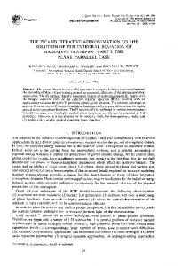
Fig. 2, Comparison of diffuse radiances obtained from a plane–parallel cloud of optical thickness 1 and rectangular clouds with the same vertical dimension but varying width-to-height ratio. Values are in normalized radiance; i.e., incoming solar flux is n cos 00. In this case 670= 0.3.
requiring the quadrature to be exact for the cos m$ and sin nrj functions, where m = O, . . .. 8 and 7. Similarly, the weights for the zenith angles, /3, are determined by requiring the n= l,..., quadrature to be exact for Legendre polynomials P~(v), k = O, . . .. m. Table 2 shows the associated weights for the specified quadrature angles.
3.2. The line integral along the characteristic In order to compute 1(”)(r, ~), the line integration is carried out along a line through r parallel to the direction Q. This path is called a characteristic. This characteristic will intersect the boundary in at least two points (i.e., at exactly two points for simple cloud geometries such as rectangular solids). At the boundary for which O points into the interior of the cloud, F’) (r, ~) is computed successively for each lattice point along the characteristic. For the lattice point at the boundary, At the first interior lattice point along the 1(”) (r, Q) is computed from the incident radiation. characteristic, only first order scattering effects are included by the line integration. At the second interior lattice point, second order scattering effects are included, and so on. Thus, by the n th interior lattice point, n th order scattering effects make a contribution. The above numerical scheme may encounter the largest error for a direction pointing into the cloud at the lattice point closest to the boundary. Although multiple scattering occurs at all points within the cloud, its importance increases with increasing values of ?. Therefore, the above integration scheme does not seriously limit the accuracy of the final result, AFurthermore, the above integration process continues along the characteristic in the direction of Q until the exiting boundary point is encountered. Therefore, the exiting radiance includes the effects of n th order multiple scattering, where n is the number of lattice points along the characteristic.
202
Kwo-Sen Kuo et al
In order to maintain the advantages of an integral equation version of the RTE over the differential equation formulation, it is necessary to use a spatial integration scheme of order greater than two (i.e., the accuracy of typical finite difference schemes). As noted above, this higher order integration scheme must be employed even for lattice points near the boundary. As the value of radiance Z@J(r, ~) is known only at lattice points, this dictates a numerical quadrature scheme based upon extrapolation. One is led to the following problem. Given a function ~(s) specified at n + 1 lattice points formula to estimate the integral s~, s,, . ..su. find an n th order quadrature “~(s)ds, J ~o
for k = 1,2 . . . ..n.
This is accomplished by constructing the unique n th degree interpolation polynomial Q,,(s), such that Qfl(sl) =~ (s{) for 1 = O, 1, . . .. n. Such a polynomial always exists, is unique, and may be computed from Lagrange interpolation. One then estimates the above integral by Sk Q.(s) ds = ~ J ~o
(6)
Wff(S,),
/=1
where w; is a weight matrix independent of ,~(sl) and depending only upon n. This approach is referred to as an extrapolation quadrature since the estimate of the integral from SOto s, involves a weighted sum of the integrand evaluated at points, some of which lie outside of the interval of integration. Choosing the order n too small will result in reduced accuracy because the quadrature error is proportional to As”. On the other hand, choosing an excessively large value of n results in a weight matrix whose entries are large and whose signs alternate. This produces numerical
Transmitted
Reflected Radianceg ;tOCloud Top Tw=rx” , I , , , I , 0.25 I , v I
Radiances at Cloud Bottom
‘oooo”oo~
— rs.o. ......D.O.-6
—
Do. . . D.O.-6 -——— 25Z -.-.–.. 44Z 0.20–..._. 69%
____25z —.—. — 44% –...
-.
/
69Z
I
I
I
j
0.10r .
Y - ,.//. “\.’
.
0.00 I 0.0
h
I t , I , , , I I , 0.2 0.4 0.6 0.6 Observation Cosine, p
! 1.0
0.01 , , I I I -1.0 -0.8
1I , ,
1
1
I I I , 1 , I 0.0 -0.6 -0.4 -0.2 Observation Cosine, p
Fig. 3. Comparison of diffuse radiances obtained from a plane-parallel cloud of optical thickness 1 and regular array of cubical clouds (t 1= 13) with varying cloud cover,
203
PI approximation—I1 Table 4. Percentage of energy leaked from the vertical boundaries for cubic clouds with different optical thicknesses, T
1
%
11.85
2 21.54
4 37.58
8 55.55
instability due to round-off error in computer arithmetic. A value of n = 11 is found to be a reasonable compromise between the need for accuracy and the necessity of avoiding numerical instabilities. Table 3 shows the weight matrix for n = 11. By increasing the value of n from 5 to 11, it is possible to increase As by a factor of five without significant loss of accuracy. This is important, as storage requirements and runtime vary inversely as AS3. 3.3. Boundary
conditions
The discussion above in Sect. 3.2, as well as the results presented below, are based upon vacuum boundary conditions. It is not difficult to incorporate other boundary conditions within the PI algorithm. To impose Lambertian or bidirectional reflectance boundary conditions at the earth’s surface requires only a slight increment in computer storage but no essential increase in computational overhead. Given a characteristic passing through a surface boundary node, integration is performed twice, once initiating at the boundary node and once terminating at that node. The modification required to implement these more complex boundary conditions entails integration along all of the characteristics terminating at the boundary node (thus obtaining the incidence radiances) before performing all those integrations along the characteristics that begin at that node. Knowledge of the incident radiances at the surface node, followed by application of the Lambertian or bidirectional reflectance conditions, yields the outgoing radiances along those same characteristics. From the perspective of cloud field radiance calculations, periodic boundary conditions must be incorporated. A cell containing one or more clouds, each of different size and optical properties, when coupled with periodic boundary conditions, represents a cloud field composed of a periodic array of such cells. Paradoxically, periodic boundary conditions lead to a slightly simpler algorithm. This occurs because all non-horizontal characteristics encounter the same number of nodes regardless of their direction; these are initiated at the top of the cell. When such a characteristic encounters a vertical boundary, it reappears from the corresponding point on the opposite face, continuing in this manner until it terminates at the lower boundary of the cell where any of the vacuum, Lambertian, or bidirectional reflectance boundary conditions may be applied. The absence of short characteristics allows one to uniformly apply high order spatial integration schemes and thus enhance the overall accuracy of the results. It is worth mentioning that if the cloud does not completely fill the periodic cell, then those nodes external to the cloud entail a nearly negligible memory and cpu requirement.
3.4. Delta function
approximation
Due to limitations in computer memory, it is difficult to treat directly realistic 3-D radiative transfer problems with a scattering phase function requiring more than about 10 Legendre expansion terms, Even aerosol phase functions frequently require more than 10 terms. In fact, it is desirable to apply the method even to cirrus phase functions requiring thousands of expansion coefficients. This, in turn, requires a modification of the PI approach which preserves highly accurate radiance calculations while reducing the demands upon memory. Although the Delta-m method developed by WiscombeiT is known to yield reasonably accurate fluxes, the radiances computed using this method exhibit oscillatory behavior and are less accurate than are the fluxes. The number of terms necessary for the phase function expansion increases with the magnitude of the forward peak. Potter18 has developed a method in which the forward peak is truncated, representing the energy missing from the forward peak by an appropriate multiple of the d-function. This method yields less accurate fluxes, but provides accurate radiances in all directions
204
Kwo-Sen Kuo et al
except near the source. Moreover, there is further benefit from the use of this approximation. scattering coefficient P, is transformed by the delta approximation as follows: P:=(I
-f)fls,
The
(7)
where ,j’ is the fraction of total scattered energy in the truncated peak, and fl~ is the effective scattering coefficient. As a consequence, the optical thickness is reduced, rendering the volume of simulation smaller and decreasing the memory requirements. In the present study, the truncation is made when the graph of the phase functions vs the scattering angle attains a slope of 30. 4.
RESULTS
Due to the fact that radiation is incident upon and exits from the sides of broken clouds, cloud shape strongly influences reflected radiances and fluxes. Although the present algorithm accommodates general cloud shapes, this investigation is limited by two simplifying assumptions: (I) clouds are homogeneous rectangular solids with a phase function corresponding to a size distribution with effective particle size of 10 pm; and (2) cloud fields are composed of regular arrays of such clouds. Results presented here fall into three categories: (1) validation of the PI 3-D algorithm utilizing plane–parallel calculations; (2) selected flux and radiance patterns for single 3-D clouds; and (3) cloud field flux and radiance patterns. 4.1. Validation The most highly accurate and widely studied solutions of the RTE are those obtained for homogeneous 1-D slabs. Thus the most sensitive test of the current PI method is obtained by comparison of radiances for a sequence of progressively wider rectangular solids with the same vertical dimension whose limit is the homogeneous slab. Figure 2 shows upward radiance patterns at the top center and downward diffuse radiance patterns at the bottom center of a sequence of rectangular solids of varying width-to-height ratios and the corresponding results for the 1-D homogeneous slab obtained from the Discrete Ordinates (DO) and delta-DO (d-DO) methods at normal incidence. As expected, the 3-D PI solution approaches the 1-D solution from below as the ratio of cloud width-to-height increases. The PI solutions at the bottom center and top center are everywhere less than the corresponding 1-D solutions. This behavior results from photons exiting the cloud sides. As the width-to-height ratio increases, a progressively smaller fraction of the incident photons escape via this route, thereby causing the 3-D PI solution to approach the 1-D DO solution over a wide range of angles. The full DO solution shown in Fig. 2 was obtained using 268 Legendre expansion coefficients in the representation of the phase function, while the d-DO solution employs 32 terms. The PI method results in returned values at each of 10 zenith angles; the DO results are computed at 132 angles, while the d-DO results are computed at 16 angles. This accounts for the somewhat coarser appearance of the d-DO and PI curves in Fig. 2. The most noticeable discrepancy between the PI and DO results in Fig. 2 occurs at ,u = 1.0 for the radiance computed at the top center of the cloud. This difference is due in large part to the transformation associated with the d-approximation applied to the PI method. The effect of this transformation is to redistribute some of the diffuse radiance in the forward direction to the direct solar beam. This discrepancy is even larger in the d-DO solution. For the radiance pattern at the bottom center of the cloud, an even larger deviation is obtained between the PI and DO solutions near v = – 1.0. This is an artifact of the scaling transformation, as well as a result of sampling the radiance field at a limited number of values. The above calculations were performed with a single scattering albedo of mO= 1. Therefore, flux conservation provides a secondary test of accuracy. In all cases, the flux conservation for the 3D d-PI method exceeds 997., From a remote sensing perspective, it is rarely the case that the satellite and the sun are in the same direction. Therefore, the difference in radiances near p = 1.0 seldom can be observed. Figure 3 shows an analogous sequence of radiance patterns generated for a cloud field composed of a regular array of cubical clouds. Similarly, as the percentage cloud cover increases, the PI solution at the center–top and center–bottom approach the corresponding plane–parallel solution.
PI approximation—II
Mean Radiances (Upward at z = 2.00 km) .“”-”””””:”””U$S--..::.. ..:...-. ....:.. ....:..” . .................... . ..... /:::..” .... ...... -..:.. .. ..+. /.-.” .. ..:.. ,..,:,:. ,..” /..-..................-... ..‘$. +....:., ..... ,,:-”.. .,.. ..... ...“... ...... ‘.... -“ ...-------------- ,..”: .. ..,. ...... /“” ,.... ......”” ...... ., .. ...*. ..-” Q ., ...,, ..,.., ..! .. . .’ .,.”” .,..,, .. .... .... .. . ;..,.,., ,,. .’ .,.,...... ..... ...”” !. ., .: “., .,. :.. ;; : : . .” ,.”’.,.;./. ... .:: . :: ;., ..,~,..’”:: ;;:: . .................. }J............. ...... ................... ........>..... Hi: \ :, ,.. : “.. .: ;., : : .. ... :: :,;.. ::,:;. ; .... ,..’ ~ ;: j { :..: : , ~> ., ,. . . .. .
I&an
205
Radiances
(Downward
at
0.00 km)
““’::.$wz~ ..:.,...%. .............* :....-----....’ ....”‘...... *.:... “.-. ... ..:..? ...... ‘... ,..:;.. ....... ------.....................-........ -’”.::::::....................-.:::-...... ............ Mean Radiances (UDward at z = 4.00 km)
Mean Radiances (Downward at 0.00 km)
Wean Radiances (bwsrd
khan Radiances (Downward at 0.00 km)
--..........
—
at z = 0.00 km)
..
J
Fig. 4, Spatially averaged diffuse radiances exiting from the top and bottom faces of single, cubical clouds. Cloud dimensions are, from toD row to bottom row. T 3 = 23,43.and 83, Radiance ~atterns are disdaved as functions of observation angie, Dotted curves portray the coordinates. Concentric circles denote’ze;ith angles in an interval of 15°, with the outermost being 90° and innermost being 15’, Radial lines denote azimuthal angles in 45° increments starting from the positive x-axis, QSRT 55,2–E
206
Kwo-Sen Kuo et al
Table 4 shows the total energy exiting the top, sides, and bottom for cubical clouds of r = 1, 2,4, and 8, and solar zenith angle of 00 = 0’. At r = 1, the majority of incident energy is transmitted through the lower boundary of the cloud; about 13 Y, is scattered out the sides. As optical thickness
Radiance
a}
at z = 8.00
km
(14)
8
6
2
0 0 b)
2
Radiance
o
2
4 X (km)
at z = 8,00
4 X (km)
Fig. 5(a) and (b),
Capfim
8
6
km
6
opposite
[ O)
8
PI approximation—Ii
c)
Radiance
at z = 8.00
207
km
(14)
a
6
-a
54
2
0 0
2
4 X (km)
6
8
Fig, 5(c). Fig. 5. Reflected radiances from the top of a single cloud cube of z = X. The illumination and viewing geometry are, respectively, (a) 00= 0’, (d, ~)= (35,3’, 45’); (b) (O.. do) = (35.3