Closer to the solution: Iterative linear solvers - CiteSeerX

Closer to the solution: Iterative linear solvers

Gene H. Golub Stanford University

Henk A. van der Vorst Utrecht University

1 Introduction The solution of dense linear systems received much attention after the second world war, and by the end of the sixties, most of the problems associated with it had been solved. For a long time, Wilkinson's \The Algebraic Eigenvalue Problem" [107], other than the title suggests, became also the standard textbook for the solution of linear systems. When it became clear that partial dierential equations could be solved numerically, to a level of accuracy that was of interest for application areas (such as reservoir engineering, and reactor diusion modeling), there was a strong need for the fast solution of the discretized systems, and iterative methods became popular for these problems. Although, roughly speaking, the successive overrelaxation methods and the rst Krylov subspace methods were developed in the same period of time, the class of Successive Overrelaxation methods became the methods of choice, since they required a small amount of computer storage. These methods were quite well understood by the work of Young [108], and the theory was covered in great detail in Varga's book [102]. This book was the source of reference for iterative methods for a long time. It may seem evident that iterative methods gained in importance as scienti c modeling led to larger linear problems, since direct methods are often too expensive in terms of computer memory and CPU-time requirements. However, the convergence behavior of iterative methods depends very much on (often a priori unknown) properties of the linear system, which means that one has to consider the origin of the problem. Since large linear systems may arise from various sources, for instance, data tting problems, discretization of PDE's, Markov chains, or tomography, these properties may also vary widely. This means that one has to study the usefulness of iterative schemes for each class of problems separately and one can hardly rely on expertise gained from other classes. Most often preconditioning is required to obtain or improve convergence. Only for some classes of problems the eects of preconditioning are well understood; for 1

2 Closer to the solution: Iterative linear solvers most problems it remains largely a matter of trial and error. In our nal section we will give some hints on preconditioning as well as pointers to literature. Also the (sparsity) structure of the matrix is important for the decision between algorithms: special algorithms can often be designed for special structures, e.g., Toeplitz matrices, banded matrices, red-black ordering, p-cyclic matrices, etc. Some important matrix properties can be easily deduced from the originating problem, for instance, symmetry and positive de niteness. Iterative methods that rely on these properties, such as the Lanczos method and the conjugate gradient method, have therefore the most widespread use. The conjugate gradient method, and the method of Lanczos, were rst viewed as exact projection methods, and since their behavior in nite precision arithmetic was not in agreement with that point of view, they were initially considered with suspicion. Through work of Reid [79], it became clear that these methods, if used as iterative techniques, could be used to advantage for many classes of linear systems. With preconditioning [21], these methods could be made even more ecient. Among the rst popular preconditioned methods was ICCG [69, 63]. In the period after 1975, we have seen that symmetric positive de nite sparse systems were usually solved by preconditioned CG methods, when very large, and by sparse direct solvers if moderately large. For inde nite symmetric sparse systems special variants were proposed, like MINRES, and SYMMLQ [74]. However, for very large unsymmetric systems, the SOR methods, and the method of Chebyshev [102, 54, 53], nicely tuned by Manteuel [68], were still the methods of choice. Due to several poorly understood numerical problems, the two-sided Lanczos method, and a special variant Bi-CG [41], were not so popular at that time, but slowly more robust variants of Krylov subspace methods, with longer recursion formulas, entered the eld. We mention GENCG [32], FOM [84], ORTHOMIN [103], ORTHODIR and ORTHORES [62]. In the mid-eighties we see the start of the popularity of Krylov subspace methods for large unsymmetric systems, and many new powerful and robust methods were proposed. The past 10 years have formed a very lively area of research for these methods, but we believe that by now this has come more or less to an end. We are now facing other challenging problems for the solution of very large sparse problems. For large linear systems, associated with 3-dimensional modeling, the iterative methods are often the only means we have for solution. Of course, for structured and rather regular problems the multigrid methods have usually a better rate of convergence, but even from the CFD community we see an increasing attention to iterative schemes. We believe that it is not fruitful to see the two classes of methods as competitive, they may be combined, where depending on the point of view, multigrid is used as a preconditioner, or the iterative scheme as a smoother. We will not further discuss multigrid in our paper; it deserves separate attention. An excellent introduction to multigrid and the related multilevel methods, in the context of solving linear systems stemming

Gene H. Golub

3

from certain classes of problems, can be found in [61]. In the next section we will highlight the Krylov subspace methods as the source of one of the most important developments in the period 1985-1995. In subsequent sections, we will discuss a number of new variants. For ease of presentation we restrict ourselves to real-valued problems. Matrices will be denoted by capitals (A, B, ...), vectors are represented in lower case (x, y, ...), and scalars are represented by Greek symbols (, , ...). Unless stated dierently, matrices will be of order n: A 2 IRnn , and vectors will have length n.

2 Krylov subspace methods: the basics The past ten years have led to well-established and popular methods, that all lead to the construction of approximate solutions in the so-called Krylov subspace. Given a linear system Ax = b, with a large, usually sparse, unsymmmetric nonsingular matrix A, then the standard Richardson iteration xk = (I , A)xk,1 + b generates approximate solutions in shifted Krylov subspaces x0 + K k (A; r0) = x0 + fr0; Ar0; : : :; Ak,1r0g; with r0 = b , Ax0, for some given initial vector x0 . The Krylov subspace projection methods fall in three dierent classes: 1. The Ritz-Galerkin approach: Construct the xk for which the residual is orthogonal to the current subspace: b , Axk ? K k (A; r0). 2. The minimum residual approach: Identify the xk for which the Euclidean norm kb , Axk k2 is minimal over K k (A; r0). 3. The Petrov-Galerkin approach: Find an xk so that the residual b , Axk is orthogonal to some other suitable k-dimensional subspace. The Ritz-Galerkin approach leads to such popular and well-known methods as Conjugate Gradients, the Lanczos method, FOM, and GENCG. The minimum residual approach leads to methods like GMRES, MINRES, and ORTHODIR. If we select the k-dimensional subspace in the third approach as K k (AT ; s0), then we obtain the Bi-CG, and QMR methods. More recently, hybrids of the three approaches have been proposed, like CGS, Bi-CGSTAB, BiCGSTAB(`), TFQMR, FGMRES, and GMRESR. Most of these methods have been proposed in the last ten years. GMRES, proposed in 1986 by Saad and Schultz [84], is the most robust of them, but, in terms of work per iteration step it is also the most expensive. Bi-CG, which

4 Closer to the solution: Iterative linear solvers was suggested by Fletcher in 1977 [41], is a relatively inexpensive alternative, but it has problems with respect to convergence: the so-called breakdown situations. This aspect has received much attention in the past period. Parlett et al [75] introduced the notion of look-ahead, in order to overcome breakdowns, and this was further perfected by Freund and Nachtigal [45], and by Brezinski and Redivio-Zaglia [12]. The theory for this look-ahead technique was linked to the theory of Pade approximations by Gutknecht [59]. Other contributions to overcome speci c breakdown situations were made by Bank and Chan [9], and Fischer [39]. We will discuss these approaches in our section on QMR. The hybrids were developed primarily in the second half of the last 10 years; the rst of these was CGS, published in 1989 by Sonneveld [89], and followed by Bi-CGSTAB, by van der Vorst in 1992 [98], and others. The hybrid variants of GMRES: Flexible GMRES and GMRESR, in which GMRES is combined with some other iteration scheme, have only been proposed very recently. A nice overview of Krylov subspace methods, with focus on Lanczos-based methods, is given in [44]. Simple algorithms and unsophisticated software for some of these methods is provided in [10]. Iterative methods with much attention to various forms of preconditioning have been described in [5]. Recently a book on iterative methods was published also by Saad [83]; it is very algorithm oriented, with, of course, a focus on GMRES and preconditioning techniques, like threshold ILU, ILU with pivoting, and incomplete LQ factorizations. An annotated entrance to the vast literature on preconditioned iterative methods is given in [14].

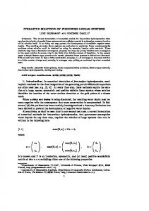
2.1 Working with the Krylov subspace In order to identify optimal approximate solutions in the Krylov subspace we need a suitable basis for this subspace, one that can be extended in a meaningful way for subspaces of increasing dimension. The obvious basis r0 , Ar0 , : : :, Ai,1 r0, for K i (A; r0), is not very attractive from a numerical point of view, since the vectors Aj r0 point more and more in the direction of the dominant eigenvector for increasing j (the power method!), and hence the basis vectors become dependent in nite precision arithmetic. Instead of the standard basis one usually prefers an orthonormal basis, and Arnoldi [1] suggested computing this basis as follows. Start with v1  r0 =kr0k2. Assume that we have already an orthonormal basis v1 , : : :, vj for K j (A; r0), then this basis is expanded by computing t = Avj , and by orthonormalizing this vector t with respect to v1 , : : :, vj . In principle the orthonormalization process can be carried out in dierent ways, but the most commonly used approach is to do this by a modi ed Gram-Schmidt procedure [53]. This leads to an algorithm for the creation of an orthonormal basis for K m (A; r0), as in Fig 1. It is easily veri ed that v1 , : : :, vm form an orthonormal basis for K m (A; r0) (that is, if the construction does not terminate at a vector t = 0). The or-

Gene H. Golub

5

v1 = r0 =kr0k2 ; for j = 1; ::; m , 1 t = Avj ; for i = 1; :::; j hi;j = viT t; t = t , hi;j vi ; end; hj +1;j = ktk2; vj +1 = t=hj +1;j ; end

Figure 1.

Arnoldi's method with modi ed Gram{Schmidt orthogonalization

thogonalization leads to relations between the vj , that can be formulated in a compact algebraic form. Let Vj denote the matrix with columns v1 up to vj , then it follows that AVm,1 = Vm Hm;m,1 : The m by m , 1 matrix Hm;m,1 is upper Hessenberg, and its elements hi;j are de ned by the Arnoldi algorithm. From a computational point of view, this construction is composed from three basic elements: a matrix vector product with A, innerproducts, and updates. We see that this orthogonalization becomes increasingly expensive for increasing dimension of the subspace, since the computation of each hi;j requires an inner product and a vector update. Note that if A is symmetric, then so is Hm,1;m,1 = VmT,1 AVm,1 , so that in this situation Hm,1;m,1 is tridiagonal. This means that in the orthogonalization process, each new vector has to be orthogonalized with respect to the previous two vectors only, since all other innerproducts vanish. The resulting three term recurrence relation for the basis vectors of Km (A; r0) is known as the Lanczos method and some very elegant methods are derived from it. In the symmetric case the orthogonalization process involves constant arithmetical costs per iteration step: one matrix vector product, two innerproducts, and two vector updates.

6

Closer to the solution: Iterative linear solvers

3 The Ritz-Galerkin approach: FOM and CG Let us assume, for simplicity, that x0 = 0, and hence r0 = b. The Ritz-Galerkin conditions imply that rk ? K k (A; r0), and this is equivalent to VkT (b , Axk ) = 0: Since b = r0 = kr0k2v1 , it follows that VkT b = kr0k2e1 with e1 the rst canonical unit vector in IRk . With xk = Vk y we obtain VkT AVk y = kr0k2e1 : This system can be interpreted as the system Ax = b projected onto K k (A; r0). Obviously we have to construct the k  k matrix VkT AVk , but this is, as we have seen, readily available from the orthogonalization process: VkT AVk = Hk;k; so that the xk for which rk ? K k (A; r0) can be easily computed by rst solving Hk;ky = kr0k2e1 , and forming xk = Vk y. This algorithm is known as FOM or GENCG. Note that for some j  n , 1 the construction of the orthogonal basis must terminate. In that case we have that AVj +1 = Vj +1Hj +1;j +1. Let y be the solution of the reduced system Hj +1;j +1y = kr0ke1 , and xj +1 = Vj +1 y. Then it follows that xj +1 = x, i.e., we have arrived at the exact solution, since Axj +1 , b = AVj +1 y , b = Vj +1 Hj +1;j +1y , b = kr0kVj +1 e1 , b = 0 (we have assumed that x0 = 0). When A is symmetric, then Hk;k reduces to a tridiagonal matrix Tk;k , and the resulting method is known as the Lanczos method [65]. In clever implementations, it is possible to avoid storing all the vectors vj . When A is in addition positive de nite then we obtain, at least formally, the Conjugate Gradient method. In commonly used implementations of this method, one implicitly forms an LU factorization for Tk;k and this leads to very elegant short recurrencies for the xj and the corresponding rj . The positive de niteness is necessary to guarantee the existence of the LU factorization, but it allows also for another useful interpretation. From the fact that ri ? K i (A; r0), it follows that A(xi , x) ? K i (A; r0), or xi , x ?A K i (A; r0). The latter observation expresses the fact that the error is A,orthogonal to the Krylov subspace and this is equivalent to the important observation that kxi , xkA is minimal1 For an overview of the history of CG and main contributions on this subject, see [51]. 1 The A,norm is de ned by ky k2 = (y; y )  (y; Ay ), and we need the positive de niteness A A of A in order to get a proper innerproduct (
;
)A.

7 The local convergence behavior of CG, and especially the occurrence of superlinear convergence, was rst explained in a qualitative sense in [21], and later in a quantitative sense in [94]. In both papers it was linked to the convergence of eigenvalues (Ritz values) of Ti;i towards eigenvalues of A, for increasing i. The global convergence can be bounded with expressions that involve condition numbers, for details see for instance [21, 53, 2]. In [2] the situation is analysed where the eigenvalues of A are in disjunct intervals. Gene H. Golub

4 The minimum residual approach The creation of an orthogonal basis for the Krylov subspace, with basis vectors v1 , : : :, vi+1 , leads to AVi = Vi+1 Hi+1;i; (4:1) where Vi is the matrix with columns v1 to vi . We look for an xi 2 K i (A; r0), that is xi = Vi y, for which kb , Axi k2 is minimal. This norm can be rewritten as kb , Axi k2 = kb , AVi yk2 = k jjr0jj2Vi+1 e1 , Vi+1 Hi+1;iyk2 : Now we exploit the fact that Vi+1 is an orthonormal transformation with respect to the Krylov subspace K i+1 (A; r0): kb , Axik2 = kkr0k2e1 , Hi+1;iyk2 ; and this nal norm can simply be minimized by solving the minimum norm least squares problem for the i + 1 by i matrix Hi+1;i and right-hand side jjr0jj2e1 . In GMRES [84] this is done eciently with Givens rotations, that annihilate the subdiagonal elements in the upper Hessenberg matrix Hi+1;i. Note that when A is Hermitian (but not necessarily positive de nite), the upper Hessenberg matrix Hi+1;i reduces to a tridiagional system. This simpli ed structure can be exploited in order to avoid storage of all the basis vectors for the Krylov subspace, in a way similar as has been pointed out for CG. The resulting method is known as MINRES [74]. In order to avoid excessive storage requirements and computational costs for the orthogonalization, GMRES is usually restarted after each m iteration steps. This algorithm is referred to as GMRES(m); the not-restarted version is often called `full' GMRES. There is no simple rule to determine a suitable value for m; the speed of convergence may vary drastically for nearby values of m. There is an interesting and simple relation between the Ritz-Galerkin approach (FOM and CG) and the minimum residual approach (GMRES and MINRES). In GMRES the projected system matrix Hi+1;i is transformed by Givens rotations to an upper triangular matrix (with last row equal to zero). So, in fact, the major dierence between FOM and GMRES is that in FOM the last ((i+1)-th row is simply discarded, while in GMRES this row is rotated to a zero

8 Closer to the solution: Iterative linear solvers vector. Let us characterize the Givens rotation, acting on rows i and i + 1, in order to zero the element in position (i + 1; i), by the sine si and the cosine ci . Let us further denote the residuals for FOM with an superscript F and those for GMRES with superscript G. Then we have the following relation between FOM and GMRES: If ck 6= 0 then the FOM and the GMRES residuals are related by

krkG k2 ; 1 , (krkGk2 =krkG,1k2)2

krkF k2 = q

(4:2)

([23]: theorem 3.1). From this relation we see that when GMRES has a signi cant reduction at step k, in the norm of the residual (i.e., sk is small, and ck  1), then FOM gives about the same result as GMRES. On the other hand when FOM has a breakdown (ck = 0), then GMRES does not lead to an improvement in the same iteration step. Because of these relations we can link the convergence behaviour of GMRES with the convergence of Ritz values (the eigenvalues of the "FOM" part of the upper Hessenberg matrix). This has been exploited in [100], for the analysis and explanation of local eects in the convergence behaviour of GMRES. There are various dierent implementations of FOM and GMRES. Among those equivalent to GMRES are: Orthomin [103], Orthodir [62], GENCR [33], and Axelsson's method [3]. These methods are often more expensive than GMRES per iteration step. Orthomin continues to be popular, since this variant can be easily truncated (Orthomin(s)), in contrast to GMRES. The truncated and restarted versions of these algorithms are not necessarily mathematically equivalent. Methods that are mathematically equivalent to FOM are: Orthores [62] and GENCG [19, 106]. In these methods the approximate solutions are constructed such that they lead to orthogonal residuals (which form a basis for the Krylov subspace; analogously to the CG method). A good overview of all these methods and their relations is given in [83]. The GMRES method and FOM are closely related to vector extrapolation methods, when the latter are applied to linearly generated vector sequences. For a discussion on this, as well as for implementations for these matrix free methods, see [85].

4.1 Inner-outer iteration schemes

Although GMRES is optimal, in the sense that it leads to a minimal residual solution over the Krylov subspace, it has the disadvantage that this goes with increasing computational costs per iteration step. Of course, with a suitable preconditioner one can hope to reduce the dimension of the required Krylov subspace to acceptable values, but in many cases such preconditioners have not been identi ed.

9 The preconditioner K ,1 is generally viewed as an approximation for the inverse of the matrix A of the system Ax = b to be solved. Instead of an optimal update direction A,1 r, we compute the direction p = K ,1 r. That is, we solve p from Kp = r, and K is constructed in such a way that this is easy to do. An attractive idea is to try to get better approximations for A,1 r, and there are two related approaches to accomplish this. One is to try to improve the preconditioner with updates from the Krylov subspace. This has been suggested rst by Eirola and Nevanlinna [31]. Their approach leads to iterative methods that are related to Broyden's method [13], which is a Newton type of method. The Broyden method can be obtained from this update-approach if we do not restrict ourselves to Krylov subspaces. See [104] for a discussion on the relation of these methods. The updated preconditioners can not be applied immediately to GMRES, since the preconditioned operator now changes from step to step, and we are not forming a regular Krylov subspace, but rather a subset of a higher dimensional Krylov subspace. However, we can still minimize the residual over this subset. The idea of variable preconditioning has been exploited in this sense, by dierent authors. Axelsson and Vassilevski [7] have proposed a Generalized Conjugate Gradient method with variable preconditioning, Saad [81, 83] has proposed a scheme very similar to GMRES, called Flexible GMRES (FGMRES), and Van der Vorst and Vuik have published a GMRESR scheme. FGMRES has received most attention, presumably because it is so easy to implement: only the update directions in GMRES have to be preconditioned, and each update may be preconditioned dierently. This means that only one line in the GMRES algorithm has to be adapted. The price to be paid is that the method is no longer robust; it may break down. The GENCG and GMRESR schemes are slightly more expensive in terms of memory requirements and in computational overhead per iteration step. The main dierence between the two schemes is that GENCG in [7] works with Gram-Schmidt orthogonalization, whereas GMRESR makes it possible to use Modi ed Gram-Schmidt. This may give GMRESR an advantage in actual computations. In exact arithmetic GMRESR and GENCG should produce the same results for the same preconditioners. Another advantage of GMRESR over Algorithm 1 in [7] is that only one matrix vector product is used per iteration step in GMRESR; GENCG needs two matrix vector products per step. In GMRESR the residual vectors are preconditioned and if this gives a further reduction then GMRESR does not break down. This gives slightly more control over the method in comparison with FGMRES. In most cases though the results are about the same, but the ecient scheme for FGMRES has an advantage. We will brie y discuss the GMRESR method. In [101] it has been shown how the GMRES-method, or more precisely, the GCR-method, can be combined with other iterative schemes. The iteration steps of GMRES (or GCR) are called outer Gene H. Golub

10 Closer to the solution: Iterative linear solvers iteration steps, while the iteration steps of the preconditioning iterative method are referred to as inner iterations. The combined method is called GMRES?, where ? stands for any given iterative scheme; in the case of GMRES as the inner iteration method, the combined scheme is called GMRESR[101]. It was shown in [26, 25], that GMRESR can be implemented in a way that avoids about 30% of the overhead in the outerloop, which makes the method about as expensive per outer iteration step as FGMRES. The GMRES? algorithm can be described as in Fig. 2.

x0 is an initial guess; r0 = b , Ax0 ; for i = 0; 1; 2; 3; ::: Let z (m) be the approximate solution of Az = ri , obtained after m steps of an iterative method. c = Az (m) (often available from the iteration method) for k = 0; :::; i , 1  = cTk c c = c , ck z (m) = z (m) , uk ci = c=kck2; ui = z (m) =kck2 xi+1 = xi + (cTi ri)ui ri+1 = ri , (cTi ri)ci if xi+1 is accurate enough then quit end

Figure 2.

The GMRES? algorithm

A sucient condition to avoid breakdown in this method (kck2 = 0) is that the norm of the residual at the end of an inner iteration is smaller than the norm of the right-hand side residual: kAz (m) , ri k2 < krik2. This can easily be controlled during the inner iteration process. If stagnation occurs, i.e. no progress at all is made in the inner iteration, then it is suggested in [101] to do one (or more) steps of the LSQR method, which guarantees a reduction (but this reduction is often very small). The idea behind these exible iteration schemes is that we explore parts of high-dimensional Krylov subspaces, hopefully determining essentially the same approximate solution that full GMRES would nd over the entire subspace, but

11 at much lower computational costs. For the inner iteration we may select any appropriate solver, for instance, one cycle of GMRES(m), since then we have also locally an optimal method, or some other iteration scheme, like for instance Bi-CGSTAB. In [26] it is proposed to keep the Krylov subspace, that is built in the inner iteration, orthogonal with respect to the Krylov basis vectors generated in the outer iteration. Under various circumstances this helps to avoid inspection of already investigated parts of Krylov subspaces in future inner iterations. The procedure works as follows. In the outer iteration process the vectors c0, ..., ci,1 build an orthogonal basis for the Krylov subspace. Let Ci be the n by i matrix with columns c0 , ..., ci,1 . Then the inner iteration process at outer iteration i is carried out with the operator Ai instead of A, and Ai is de ned as Ai = (I , Ci CiT )A: (4:3) Of course, I , Ci CiT can be stored as a product of Householder transformations, which makes the updates more ecient. It is easily veri ed that Ai z ? c0 ; :::; ci,1 for all z, so that the inner iteration process takes place in a subspace orthogonal to these vectors. The additional costs, per iteration of the inner iteration process, are i inner products and i vector updates. In order to save on these costs, one should realize that it is not necessary to orthogonalize with respect to all previous c-vectors, and that \less eective" directions may be dropped, or combined with others. In [72, 8, 26] suggestions are made for such strategies. Of course, these strategies are only attractive in cases where we see too little residual reducing eect in the inner iteration process in comparison with the outer iterations of GMRES?. Note that if we carry out the preconditioning by doing a few iterations of some other iteration process, then we have inner-outer iteration schemes; these have been discussed earlier in [52]. It is dicult to analyse their convergence behavior and in a rst attempt it is wise to look at the analysis for simpli ed schemes. We will give the avor of this analysis and the type of results [52]. We consider a simpli ed inner-outer iteration scheme associated with the standard iteration for the splitting A = M , N, as given in Fig. 3; the inner iterations are carried out with M. With ek  x , xk , it follows that ek+1 = (I , M ,1A)ek , M ,1qk ; and kek+1 k  kI , M ,1Akkek k + kM ,1qk k  (kI , M ,1Ak + k kM ,1 kkAk)kek k: Hence kek k  ,kI , M ,1Ak + 
k ; ke k Gene H. Golub

0

12

Closer to the solution: Iterative linear solvers

while kkqrkkkk22 < k do rk = b , Axk Solve Mz = ri approximately ) zk (qk  M zk , rk ) xk = xk + zk if xk is accurate enough then quit end +1

+1

Figure 3.

A simpli ed Inner-Outer iteration scheme

with   maxk kM ,1kkAk, so that the convergence is largely determined by the norm of I , M ,1 A, if k is small enough. It can be shown that for k = k , for a xed 0 <  < 1: 

lim sup kkeek kk 0 k!1

 k1

= kI , M ,1 Ak;

so that essentially the convergence rate for the splitting A = M , N, with exact inversion of M, is restored. A similar analysis can be carried out in relation with Chebyshev acceleration, see [52, 49]. In [49] the question is studied how  can be chosen so that the total amount of work is minimized. For an application of inner-outer iterations for Stokes problems, see the inexact Uzawa scheme, proposed in [36]; for Navier-Stokes related problems, see [55].

5 The Petrov-Galerkin approach: Bi-CG For unsymmetric systems we can, in general, not reduce the matrix A to a symmetric system in a lower-dimensional subspace, by orthogonal projections. The reason is that we can not create an orthogonal basis for the Krylov subspace by a 3-term recurrence relation [38]. We can, however, try to obtain a suitable non-orthogonal basis with a 3-term recurrence, by requiring that this basis is orthogonal with respect to some other basis. We start by constructing an arbitrary basis for the Krylov subspace: hi+1;i vi+1 = Avi ,

i X j =1

hj;ivj ;

(5:1)

13 which can be rewritten in matrix notation as AVi = Vi+1 Hi+1;i. The coecients hi+1;i de ne the norm of vi+1 , and a natural choice would be to select them such that kvi+1 k2 = 1. In Bi-CG implementations, a popular choice is to select hi+1;i such that kvi+1k2 = kri+1 k2. Clearly, we can not use Vi for the projection, but suppose we have a Wi for which WiT Vi = Di (an i by i diagonal matrix with diagonal entries di ), and for which WiT vi+1 = 0. Then WiT AVi = Di Hi;i; (5:2) and now our goal is to nd a Wi for which Hi;i is tridiagonal. This means that ViT AT Wi should be tridiagonal too. This last expression has a similar structure as the right-hand side in (5.2), with only Wi and Vi reversed. This suggests to generate the wi with AT . We start with an arbitrary w1 6= 0, such that w1T v1 6= 0. Then we generate v2 with (5.1), and orthogonalize it with respect to w1, which means that h1;1 = w1T Av1 =(w1T v1 ). Since w1T Av1 = (AT w1)T v1 , this implies that w2, generated with h2;1w2 = AT w1 , h1;1w1 ; is also orthogonal to v1. This can be continued, and we see that we can create bi-orthogonal basis sets fvj g, and fwj g, by making the new vi orthogonal to w1 up to wi,1, and then by generating wi with the same recurrence coecients, but with AT instead of A. Now we have that WiT AVi = Di Hi;i, and also that ViT AT Wi = Di Hi;i. This implies that Di Hi;i is symmetric, and hence Hi;i is a tridiagonal matrix, which gives us the desired 3-term recurrence relation for the vj 's, and the wj 's. Note that v1 ; : : :; vi form a basis for K i (A; v1 ),and w1 , : : :, wi form a basis for K i (AT ; w1). We may proceed in a similar way as in the symmetric case: AVi = Vi+1 Ti+1;i ; (5:3) but here we use the matrix Wi = [w1; w2; :::; wi] for the projection of the system WiT (b , Axi ) = 0; or WiT AVi y , WiT b = 0: Using (5.3), we nd that yi satis es Ti;iy = kr0 k2e1 ; and xi = Vi y. The resulting method is known as the Bi-Lanczos method [65]. We have assumed that di 6= 0, that is wiT vi 6= 0. The generation of the biorthogonal basis breaks down if for some i the value of wiT vi = 0, this is referred Gene H. Golub

14 Closer to the solution: Iterative linear solvers to in literature as a serious breakdown. Likewise, when wiT vi  0, we have a nearbreakdown. The way to get around this diculty is the so-called Look-ahead strategy, which comes down to taking a number of successive basis vectors for the Krylov subspace together and to make them blockwise bi-orthogonal. This has been worked out in detail in [75, 45, 46, 47]. Another way to avoid breakdown is to restart as soon as a diagonal element gets small. Of course, this strategy looks surprisingly simple, but one should realise that at a restart the Krylov subspace, that has been built up so far, is thrown away, and this destroys the possibility of faster (i.e., superlinear) convergence. We can try to construct an LU-decomposition, without pivoting, of Ti;i . If this decomposition exists, then, similar to CG, it can be updated from iteration to iteration and this leads to a recursive update of the solution vector, which avoids saving all intermediate r and w vectors. This variant of Bi-Lanczos is usually called Bi-Conjugate Gradients, or for short Bi-CG [41]. In Bi-CG, the di are chosen such that vi = ri,1, similarly to CG. Of course one can in general not be certain that an LU decomposition (without pivoting) of the tridiagonal matrix Ti;i exists, and this may lead also to breakdown (a breakdown of the second kind), of the Bi-CG algorithm. Note that this breakdown can be avoided in the Bi-Lanczos formulation of the iterative solution scheme, e.g., by making an LU-decomposition with 2 by 2 block diagonal elements [9]. It is also avoided in the QMR approach (see Section 5.1). Note that for symmetric matrices Bi-Lanczos generates the same solution as Lanczos, provided that w1 = r0, and under the same condition Bi-CG delivers the same iterands as CG for positive de nite matrices. However, the Bi-orthogonal variants do so at the cost of two matrix vector operations per iteration step. For a computational scheme for Bi-CG, without provisions for breakdown, see [10].

5.1 QMR

The QMR method [47] relates to Bi-CG in a similar way as MINRES relates to CG. We start with the recurrence relations for the vj : AVi = Vi+1 Ti+1;i : We would like to identify the xi, with xi 2 K i (A; r0), or xi = Vi y, for which kb , Axi k2 = kb , AVi yk2 = kb , Vi+1 Ti+1;i yjj2 is minimal, but the problem is that Vi+1 is not orthogonal. However, we pretend that the columns of Vi+1 are orthogonal. Then kb , Axik2 = kVi+1 (kr0k2e1 , Ti+1;i y)k2 = k(kr0k2e1 , Ti+1;iy)k2 ;

15 and in [47] it is suggested to solve the projected miniminum norm least squares problem k(kr0k2 e1 , Ti+1;i y)k2 . The minimum value of this norm is called the quasi residual and will be denoted by jjriQjj2. Since, in general, the columns of Vi+1 are not orthogonal, the computed xi = Vi y does not solve the minimum residual problem, and therefore this approach is referred to as a Quasi-minimum residual approach [47]. It can be shown that the norm of the residual riQMR of QMR can be be bounded in terms of the quasi residual p jjriQMRjj2  i + 1 jjriQjj2: The sketched approach leads to the simplest form of the QMR method. A more general form arises if the least squares problem is replaced by a weighted least squares problem [47]. No strategies are yet known for optimal weights. In [47] the QMR method is carried out on top of a look-ahead variant of the biorthogonal Lanczos method, which makes the method more robust. Experiments indicate that although QMR has a much smoother convergence behaviour than Bi-CG, it is not essentially faster than Bi-CG. This is con rmed explicitly by the following relation for the Bi-CG residual rkB and the quasi residual rkQ (in exact arithmetic): krkQk2 krkB k2 = q ; 1 , (krkQ k2 =krkQ,1k2)2 see [23]: Theorem 4.1. This relation, which is similar to the relation for GMRES and FOM, shows that when QMR gives a signi cant reduction at step k, then Bi-CG and QMR have arrived at residuals of about the same norm (provided, of course, that the same set of starting vectors has been used). It is tempting to compare QMR with GMRES, but this is dicult. GMRES really minimizes the 2-norm of the residual, but at the cost of increasing the work of keeping all residuals orthogonal and increasing demands for memory space. QMR does not minimize this norm, but often it has a convergence comparable to GMRES, at a cost of twice the amount of matrix vector products per iteration step. However, the generation of the basis vectors in QMR is relatively cheap and the memory requirements are limited and modest. In view of the relation between GMRES and FOM, it will be no surprise that there is a similar relation between QMR and Bi-CG, for details of this see [47]. This relation expresses that at a signi cant local error reduction of QMR, Bi-CG and QMR have arrived almost at the same residual vector (similar to GMRES and FOM). However, QMR is preferred to Bi-CG in all cases because of its much smoother convergence behaviour, and also because QMR removes one break-down condition (even when implemented without look-ahead). Several variants of QMR, or rather Bi-CG, have been proposed, which increase the eectiveness of this class of methods in certain circumstances. In a recent paper, Zhou and Walker [110] have shown that the Quasi-Minimum Gene H. Golub

16 Closer to the solution: Iterative linear solvers Residual approach can be followed for other methods, such as CGS and BiCGSTAB, as well. The main idea is that in these methods the approximate solution is updated as xi+1 = xi + ipi ; and the corresponding residual is updated as ri+1 = ri , iApi : This means that APi = Wi Ri+1 , with Wi a lower bidiagonal matrix. The xi are combinations of the pi , so that we can try to nd the combination Piyi for which kb , APiyi k2 is minimal. If we insert the expression for APi , and ignore the fact that the ri are not orthogonal, then we can minimize the norm of the residual in a quasi-minimum least squares sense, similar to QMR.

5.2 CGS

It is well known that the bi-conjugate gradient residual vector can be written as rj (= j vj ) = Pj (A)r0 , and, likewise, the so-called shadow residual r^j (= j wj ) can be written as r^j = Pj (AT )^r0. Because of the bi-orthogonality relation we have that (rj ; r^i) = (Pj (A)r0 ; Pi(AT )^r0) = (Pi(A)Pj (A)r0 ; r^0) = 0; for i < j. The iteration parameters for bi-conjugate gradients are computed from innerproducts like the above. Sonneveld [89] observed that we can also construct the vectors r~j = Pj2 (A)r0, using only the latter form of the innerproduct for recovering the bi-conjugate gradients parameters (which implicitly de ne the polynomial Pj ). By doing so, the computation of the vectors r^j can be avoided and so can the multiplication by the matrix AT . The resulting CGS [89] method works in general very well for many unsymmetric linear problems. It converges often much faster than BI-CG (about twice as fast in some cases) and has the advantage that fewer vectors are stored than in GMRES. These three methods have been compared in many studies (see, e.g., [78, 15, 76, 71]). CGS, however, usually shows a very irregular convergence behaviour. This behaviour can even lead to cancellation and a \spoiled" solution [98]; see also Section 5.3. Freund [48] suggested a squared variant of QMR, which was called TFQMR. His experiments show that TFQMR is not necessarily faster than CGS, but it has certainly a much smoother convergence behavior.

5.3 How serious is irregular convergence?

By very irregular convergence we refer to the situation where successive residual vectors in the iterative process dier in orders of magnitude in norm, and some of these residuals may even be much larger in norm than the starting residual.

17 We will give an indication why this is a point of concern, even if eventually the (updated) residual satis es a given tolerance. For more details we refer to Sleijpen et al [86, 87]. We say that an algorithm is accurate for a certain problem if the updated residual rj and the true residual b , Axj are of comparable size for the j's of interest. In most iteration schemes the approximation for the solution and the corresponding residual are updated independently: xj +1 = xj + wj +1 rj +1 = rj , Awj +1 : In nite precision arithmetic, there will at least be a discrepancy between the two updated quantities due to the multiplication by A. We can account for that by writing rj +1 = rj , Awj +1 ,
A wj +1 for each j; (5:4) where
A is an n  n matrix for which j
Aj  nA  jAj: nA is the maximum number of non-zero matrix entries per row of A, jB j  (jbij j) if B = (bij ),  is the relative machine precision, the inequality  refers to element-wise . Note that we have ignored the nite precision errors due to the vector additions. In this case (i.e. situation (5.4) whenever we update the approximation), we have that Gene H. Golub

rk , (b , Axk ) =

k X j =1


A wj =

k X j =1


A (ej ,1 , ej );

(5:5)

where the perturbation matrix
A may depend on j and ej is the approximation error in the jth approximation: ej  x , xj . Hence, kej k jkrk k , kb , Axk kj  2k nA  kjAjk max j

 2k nA  kjAjk A,1 max krj k: (5.6) j

Except for the factor k, the rst upper{bound appears to be rather sharp. We see that approximations with large approximation errors may ultimately lead to an inaccurate result. Such large local approximation errors are typical for CGS; Van der Vorst[98] describes an example of the resulting numerical inaccuracy. If there are a number of approximations with comparable large approximation errors, then their multiplicity may replace the factor k; otherwise it will be only the largest approximation error that makes up virtually the bound for the deviation. A more rigorous analysis, leading to essentially the same results, has been given by Greenbaum [56]. She also includes the errors introduced by the multiplication and subtraction in ri+1 = ri , iAwi . However, the qualitative results

18 Closer to the solution: Iterative linear solvers of this analysis are the same, since in general the errors in the matrix vector product dominate.

5.4 Bi-CGSTAB

Bi-CGSTAB [98] is based on the following observation. Instead of squaring the Bi-CG polynomial, we can construct other iteration methods, by which xi are ~ An generated so that ri = P~i(A)Pi (A)r0 with other ith degree polynomials P. ~ obvious possibility is to take for Pj a polynomial of the form

Qi (x) = (1 , !1x)(1 , !2x):::(1 , !i x); (5:7) and to select suitable constants !j . This expression leads to an almost trivial recurrence relation for the Qi. In Bi-CGSTAB !j in the j th iteration step is chosen as to minimize rj , with respect to !j , for residuals that can be written as rj = Qj (A)Pj (A)r0 . Bi-CGSTAB needs two innerproducts more per iteration than CGS. Bi-CGSTAB can be viewed as the product of Bi-CG and GMRES(1), or rather GCR(1). Of course, other product methods can be formulated as well, and this will be the subject of the next subsection. 5.4.1 Variants of Bi-CGSTAB Because of the local minimization, Bi-CGSTAB displays a much smoother convergence behavior than CGS, and more surprisingly it often also converges (slightly) faster. One weak point in Bi-CGSTAB is that there is a break-down if !j = 0. One may also expect negative eects when !j is small. As soon as the GCR(1) step in Bi-CGSTAB (nearly) stagnates, then the BiCG part in the next iteration step cannot (or can only poorly) be constructed. Another dubious aspect of Bi-CGSTAB is that the factor Qk has only real roots by construction. It is well-known that optimal reduction polynomials for matrices with complex eigenvalues may have complex roots as well. If, for instance, the matrix A is real skew-symmetric, then GCR(1) stagnates forever, whereas a method like GCR(2) (or GMRES(2)), in which we minimize over two combined successive search directions, may lead to convergence, and this is mainly due to the fact that then complex eigenvalue components in the error can be eectively reduced. This point of view was taken in [60] for the construction of the Bi-CGSTAB2 method. In the odd-numbered iteration steps the Q-polynomial is expanded by a linear factor, as in Bi-CGSTAB, but in the even-numbered steps this linear factor is discarded, and the Q-polynomial from the previous even-numbered step is expanded by a quadratic 1 , k A , k A2 . For this construction the information from the odd-numbered step is required. It was anticipated that the introduction of quadratic factors in Q might help to improve convergence for systems with complex eigenvalues, and, indeed, some improvement has been observed in practical situations (see also [77]).

19 In [88], another and even simpler approach was taken to arrive at the desired even-numbered steps, without the necessity of the construction of the intermediate Bi-CGSTAB-type step in the odd-numbered steps. In this approach the polynomial Q is constructed straight-away as a product of quadratic factors. In fact, it is shown in [88] that the polynomialQ can also be constructed as the product of `-degree factors, without the construction of the intermediate lower degree factors. The main idea is that ` successive Bi-CG steps are carried out, where for the sake of an AT -free construction the already available part of Q is expanded by simple powers of A. This means that after the Bi-CG part of the algorithm, vectors from the Krylov subspace s; As; A2 s; :::; A`s, with s = Pk (A)Qk,` (A)r0 are available, and it is then relatively easy to minimize the residual over that particular Krylov subspace. There are variants of this approach in which more stable bases for the Krylov subspaces are generated [87], but for low values of ` a standard basis satis es, together with a minimum norm solution obtained through solving the associated normal equations (which requires the solution of an ` by ` system. In most cases Bi-CGSTAB(2) will already give nice results for problems where Bi-CGSTAB may fail. Gene H. Golub

5.5 Other product methods

In the paper by Sonneveld [89], it was made clear that we can construct product methods for which rk = Hk (A)Pk (A)r0, in which Pk denotes the Bi-CG iteration polynomial, and Hk is any other arbitrary monic polynomial of exact degree k, and he showed that this can be done with the same number of matrix vector multiplications as in k steps of Bi-CG. CGS and the Bi-CGSTAB methods are special instances of these hybrid Bi-CG schemes, but other product methods have been proposed as well. In [42] it was suggested to take for Hk Bi-CG-like polynomials in an attempt to keep attractive convergence aspects of CGS, while avoiding the irregular convergence behavior. One idea is to take for Hk the Bi-CG polynomial obtained with a dierent starting vector w1 , which can be done for virtually no additional costs in Bi-CG; this leads to a generalized CGS process. Another idea is to take for Hk the product of Pk,1 and a suitable xed rst degree factor. The idea is that the zeros of Pk and Pk,1 do not coincide, so that it is likely that a zero of Pk,1 will be close to a local maximum of Pk . This avoids the squaring eects in CGS, while it maintains the desired squaring eects in converged eigendirections. Both ideas are easily implemented in an existing CGS code. In [109] it is suggested to generate Hk by a three term recurrence relation. This leads to an expression for rk of the form rk = tk,1 , k,1yk,1 , k,1Atk,1; where tk,1 and yk,1 are auxiliary vectors in the hybrid Bi-CG iteration process, and k,1 and k,1 represent the coecients in a Bi-CG like three term recurrence

20 Closer to the solution: Iterative linear solvers for Hk . The idea suggested in [109] is to minimize the Euclidean norm of rk as a function of k,1 and k,1, and this leads to product methods which, according to given examples, can compete with CGS and Bi-CGSTAB methods. It is not clear whether these generalized product methods oer an advantage over the higher order Bi-CGSTAB(`) methods.

6 Preconditioning In order to improve the speed of convergence of iterative methods, one applies usually some form of preconditioning. Many dierent preconditioners have been suggested over the years, each of these preconditioners more or less successful for restricted classes of problems. Among all these preconditioners the Incomplete LU factorizations [69, 21] are the most popular ones, and attempts have been made to improve them, for instance by including more ll [70], or by modifying the diagonal of the ILU factorization in order to force rowsum constraints [58, 6, 5, 73, 95, 34], or by changing the ordering of the matrix [96, 97]. A collection of experiments with respect to the eects of ordering is contained in [30]. More recently, it was discovered that a multigrid-inspired ordering can be very eective for discretized diusion-convection equations, leading in some cases to almost grid-independent speeds of convergence [93, 11], see also [24]. In these publications the ordering strategy is combined with a drop-tolerance strategy for discarding small enough ll-in elements. Red-black ordering is an obvious approach to improve parallel properties for well-structured problems, but it got a bad reputation from experiments, like those reported in [30]. If carefully done though, they can lead to signi cant gains in eciency. Elman and Golub [35] suggested such an approach, in which Red-Black ordering was combined with a reduced system technique. The idea is simple, eliminate the red points, and construct an ILU for the reduced system of black points. Recently, DeLong and Ortega [28] suggested carrying out a few steps of red-black ordered SOR as a preconditioner for GMRES and Bi-CGSTAB. The key to success in these cases seems to be combined eect of fast convergence of SOR for red-black ordering, and the ability of the Krylov subspace to remove stagnations in convergence behaviour associated with a few isolated eigenvalues of the preconditioned matrix. Saad [80] has proposed some interesting variants on the incomplete LU approach for the matrix A, one of which is in fact an incomplete LQ decomposition. In this approach it is not necessary to form the matrix Q explicitly, and it turns out that the lower triangular matrix L can be viewed as the factor of an incomplete Choleski factorization of the matrix AT A. This can be exploited in the preconditoning step, avoiding the use of Q. The second approach was to introduce partial pivoting in ILU, which appears to have some advantages for convection-dominated problems. This approach was further improved by includ-

Gene H. Golub

21

ing a threshold technique for ll-in [82]. Another major step forward, for important classes of problems, was the introduction of block variants of incomplete factorizations [92, 20, 4], and modi ed variants of them [4, 66]. It was observed, by Meurant, that these block variants were more successful for discretized 2-dimensional problems than for 3-dimensional problems, unless the `2-dimensional' blocks in the latter case were solved accurately. For discussions and analysis on ordering strategies, in relation to modi ed block incomplete factorizations, see [67]. Domain decomposition methods were motivated by parallel computing, but it appeared that the approach could be used with success also for the construction of preconditioners. Domain decomposition has been used for problems that arise from discretization of a PDE over a given domain. The idea is to split the given domain into subdomains, and to solve the discretized PDE's over each subdomain separately. The main problem is to nd proper boundary conditions along the interior boundaries of the subdomains. Domain decomposition is used in an iterative fashion and usually the interior boundary conditions are based upon information on the approximate solution of neighboring subdomains that is available from a previous iteration step. It was shown by Chan and Goovaerts [17] that domain decomposition can actually lead to improved convergence rates, provided the number of domains is not too large. A splitting of the matrix with overlapping subblocks along the diagonal, which can be viewed as a splitting of the domain, if the matrix is associated with a discretized PDE and has been ordered properly, was suggested by Radicati and Robert [78]. They suggested to construct incomplete factorizations for the sub-blocks. These sub-blocks are then applied to corresponding parts of the vectors involved, and some averaging was applied on the overlapping parts. A more sophisticated domain-oriented splitting was suggested in [105], for SSOR and MILU decompositions, with a special treatment for unknowns associated with interfaces between the subdomains. The isolation of sub-blocks was done by Tang [91] in such a way that the sub-blocks corresponded to subdomains with proper internal boundary conditions. In this case it is necessary to modify the sub-blocks of the original matrix such that the subblocks could be interpreted as the discretizations for subdomains with Dirichlet and Neumann boundary conditions in order to force some smoothness of the approximated solution across boundaries. In [90] this was further improved by requiring also continuity of cross-derivatives of the approximate solution across boundaries. The local ne-tuning of the resulting interpolation formulae for the discretizations was carried out by local Fourier-analysis. It was shown that this approach could lead to impressive reductions in numbers of iterations for convection dominated problems. Another approach that received attention is the concept of constructing an

22 Closer to the solution: Iterative linear solvers explicit approximation for the inverse of a given matrix A. The idea is to nd a sparse matrix M such that kAM , I k is small for some convenient norm. Kolotilina and Yeremin [64] presented an algorithm in which the inverse was delivered in factored form, which has the advantage that singularity of M can be easily detected. In [22] an algortithm is presented which uses the 1-norm for the minimization. We also mention Chow and Saad [18], who use GMRES for the minimization of kAM , I kF . This approach has the disadvantage that one does not have easy control over the amount of ll-in in M, and drop-tolerance strategies have to be applied. The approach has the advantage that it can be used to correct explicitly some given implicit approximation, like for instance an ILU decomposition. An elegant approach was suggested by Grote and Huckle [57]. They also attempt to minimize the F-norm, which is equivalent to the Euclidean norm for the errors in the columns mi of M:

kAM , I k2F =

n X i=1

jjAmi , ei k22:

Based on this observation they derive an algorithm that produces the sparsity pattern for the most error-reducing elements of M. This is done in steps, starting with a diagonal approximation, each steps adds more non-zero entries to M, and the procedure is stopped when the norms are small enough or when memory requirements are violated.

7 Quo Vadis? In the previous sections we have seen a large number of new iterative methods, which have come in addition to older methods like Richardson's method, GaussJacobi, Gauss-Seidel, SOR, SSOR, BSOR, S2LOR, Chebyshev iteration, and many more. From the positive point of view, this huge variety in methods has provided us with a powerful toolbox from which we can select the appropriate tool for a given problem. From the point of view of the poor user however, this toolbox is confusingly large. In many practical situations it is not clear at all what method to select. One is often faced with the question from outside the expert community which method is the best, but there is in general no best method. This is nicely illustrated in [71], where examples are given of dierent types of linear systems with quite dierent convergence behavior for a few archetypes of the methods discussed before. It is shown that for each method there is a linear system for which the given method is the clear winner, as well as a linear system for which the same method is the clear looser. For instance, there is an example for which the, in general slowly converging, LSQR method is better than the, in general fast converging, GMRES method by orders of magnitudes. This also puts the eorts in perspective where the methods are compared on the basis of some examples. Hopefully this gives us some insight

23 in the properties of these methods, but what we really need is some insight into the characteristics of the linear systems that discriminate between methods. At present the situation is even more complicated due to the existence of distributed memory parallel computers. These architectures can be used eciently only if one succeeds in keeping communication between processors below certain levels, and it turns out that the innerproducts, which are needed for the Krylov subspace methods, become a bottleneck for the eciency for larger numbers of processors [27]. This has led to a revival of interest in innerproduct-free methods, like Chebyshev's method and SOR. It has been suggested to use these methods in combination with the Krylov subspace methods (as a polynomial preconditioner, see [53, 83] for discussions on this), see also our section on preconditioning. An interesting approach to construct an innerproduct-free variant of CG from information obtained after a few steps of CG is hinted in [40], where orthogonal polynomials are constructed based on partial information obtained from CG-iteration polynomials. It has been shown by Golub and Kent [50] that the optimal parameters for the Chebyshev method can also be deduced from the Chebyshev iteration vectors. This has been further worked out by Calvetti et al [16], who show how adaptive Chebyshev methods can be constructed with iteration parameters that are obtained as in [50]. It is well-known that the distribution of eigenvalues has to do with the speed of convergence of Krylov subspace methods, and a way to improve this distribution is known as Preconditioning. With a good preconditioner there is not much dierence between the various Krylov subspace methods, but this shifts the problem to the identi cation and construction of good preconditioners. Although much work has been done in this area, there is still a strong need for identifying good preconditioners, in particular for highly non-normal matrices and for inde nite problems. These problems play an important role in Computational Fluid Dynamics, and also Helmholtz problems lead to inde nite problems. For particular cases, for instance the Stokes problem, eective inde nite preconditioners have been proposed [55, 37]. The main diculty in inde nite preconditioning can be explained as follows. The Krylov subspace methods converge fast when the eigenvalues are clustered, say around 1. This means that the preconditioner, often viewed as an approximation to the inverse of the given matrix, must transfer the eigenvalues to 1. It may easily happen that, due to approximation errors that are intentionally made in order to keep the process ecient, eigenvalues are transferred to values close to 0. In that case the convergence of Krylov subspace methods will be slow, and it may happen that the unpreconditioned iteration process converges faster than the preconditioned iteration. Complex-valued problems can be treated as the problems discussed in this paper, in particular Hermitian problems can be treated as real symmetric ones, by replacing AT by AH , and by the appropriate change of innerproduct. Some Gene H. Golub

24 Closer to the solution: Iterative linear solvers problems, for instance in Electromagnetics, lead to symmetric complex matrices. Krylov subspace methods that take advantage of this property have been suggested in [43, 99], but preconditioning for this type of problems has remained an open problem. The approximation error in iterative schemes is not directly available, and has to be estimated or bounded in terms of information obtained in the iteration process. This can be done for special cases, for instance for the Conjugate Gradient method (see [10] and references therein). For most cases, however, the problem of getting realistic error bounds is yet unsolved. In some applications we need information on errors in speci ed components of the solution, this is also mainly an open problem. Parallel computing is a very important issue in solving large linear systems, but we have treated this issue only in passing. One might easily dedicate an entire paper for highlighting developments in this area. We restrict ourselves to referring to the overview paper by Demmel et al [29], in which parallel approaches are discussed as well as open problems in this area. Although the list of interesting open problems can be made arbitrarily longer, space limitations forced us to mention only a few of them.

Acknowledgements

The authors wish to thank Andy Wathen for his careful reading of the manuscript, which has helped in improving the presentation. The work of Gene H. Golub was in part supported by the National Science Foundation, Grant Number CCR-9505393. The work of Henk A. Van der Vorst was in part supported by the Dutch Research Organization NWO, MPR cluster project 95MPR04.

Bibliography 1. W. E. Arnoldi. The principle of minimized iteration in the solution of the matrix eigenproblem. Quart. Appl. Math., 9:17{29, 1951. 2. O. Axelsson. Solution of linear systems of equations: iterative methods. In V. A. Barker, editor, Sparse Matrix Techniques, Berlin, 1977. Copenhagen 1976, Springer Verlag. 3. O. Axelsson. Conjugate gradient type methods for unsymmetric and inconsistent systems of equations. Lin. Alg. Appl., 29:1{16, 1980. 4. O. Axelsson. A general incomplete block-factorization method. Lin. Alg. Appl., 74:179{190, 1986. 5. O. Axelsson. Iterative Solution Methods. Cambridge University Press, Cambridge, 1994.

25 O. Axelsson and G. Lindskog. On the eigenvalue distribution of a class of preconditioning methods. Numer. Math., 48:479{498, 1986. O. Axelsson and P. S. Vassilevski. A black box generalized conjugate gradient solver with inner iterations and variable-step preconditioning. SIAM J. Matrix Anal. Appl., 12(4):625{644, 1991. Z. Bai, D. Hu, and L. Reichel. A Newton basis GMRES implementation. IMA J. Numer. Anal., 14:563{581, 1991. R. E. Bank and T. F. Chan. An analysis of the composite step biconjugate gradient method. Num. Math., 66:295{319, 1993. R. Barrett, M. Berry, T. Chan, J. Demmel, J. Donato, J. Dongarra, V. Eijkhout, R. Pozo, C. Romine, and H. van der Vorst. Templates for the Solution of Linear Systems: Building Blocks for Iterative Methods. SIAM, Philadelphia, PA, 1994. E.F.F. Botta and A. van der Ploeg. Nested grids ILU-decomposition (NGILU). J. of Comput. and Appl. Math., 66:515{526, 1996. C. Brezinski and M. Redivo-Zaglia. Treatment of near breakdown in the CGS algorithm. Numerical Algorithms, 7:33{73, 1994. G. C. Broyden. A new method of solving nonlinear simultaneous equations. Comput. J., 12:94{99, 1969. A.M. Bruaset. A Survey of Preconditioned Iterative Methods. Longman Scienti c & and Technical, Harlow, UK, 1995. G. Brussino and V. Sonnad. A comparison of direct and preconditioned iterative techniques for sparse unsymmetric systems of linear equations. Int. J. for Num. Methods in Eng., 28:801{815, 1989. D. Calvetti, G. H. Golub, and L. Reichel. Adaptive Chebyshev iterative methods for nonsymmetric linear systems based on modi ed moments. Numerische Mathematik, 67:21{40, 1994. T.F. Chan and D.Goovaerts. A note on the eciency of domain decomposed incomplete factorizations. SIAM J. Sci. Stat. Comp., 11:794{803, 1990. E. Chow and Y. Saad. Approximate inverse preconditioners for general sparse matrices. Technical Report Research Report UMSI 94/101, University of Minnesota Supercomputing Institute, Minneapolis, Minnesota, 1994. P. Concus and G. H. Golub. A generalized Conjugate Gradient method for nonsymmetric systems of linear equations. Technical Report STANCS-76-535, Stanford University, Stanford, CA, 1976. Gene H. Golub

6. 7. 8. 9. 10.

11. 12. 13. 14. 15. 16. 17. 18.

19.

26 Closer to the solution: Iterative linear solvers 20. P. Concus, G. H. Golub, and G. Meurant. Block preconditioning for the conjugate gradient method. SIAM J. Sci. Stat. Comput., 6:220{252, 1985. 21. P. Concus, G. H. Golub, and D. P. O'Leary. A generalized conjugate gradient method for the numerical solution of elliptic partial dierential equations. In J. R. Bunch and D. J. Rose, editors, Sparse Matrix Computations. Academic Press, New York, 1976. 22. J. D. F. Cosgrove, J. C. Diaz, and A. Griewank. Approximate inverse preconditionings for sparse linear systems. Intern. J. Computer Math., 44:91{110, 1992. 23. J. Cullum and A. Greenbaum. Relations between Galerkin and normminimizing iterative methods for solving linear systems. SIAM J. Matrix Anal. Appl., 17:223{247, 1996. 24. E. F. D'Azevedo, F. A. Forsyth, and W. P. Tang. Ordering methods for preconditioned conjugate gradient methods applied to unstructured grid problems. SIAM J. Matrix Anal. Appl., 13:944{961, 1992. 25. E. De Sturler. Nested Krylov methods based on GCR. J. of Comput. Appl. Math., 67:15{41, 1996. 26. E. De Sturler and D. R. Fokkema. Nested Krylov methods and preserving the orthogonality. In N. Duane Melson, T.A. Manteuel, and S.F. McCormick, editors, Sixth Copper Mountain Conference on Multigrid Methods, volume Part 1 of NASA Conference Publication 3324, pages 111{126. NASA, 1993. 27. E. De Sturler and H.A. Van der Vorst. Reducing the eect of global communication in GMRES(m) and CG on parallel distributed memory computers. J. Appl. Num. Math., 18:441{459, 1995. 28. M. A. DeLong and J. M. Ortega. SOR as a preconditioner. J. Appl. Num. Math., 18:431{440, 1995. 29. J. Demmel, M. Heath, and H. Van der Vorst. Parallel numerical linear algebra. In Acta Numerica 1993. Cambridge University Press, Cambridge, 1993. 30. I. S. Du and G. A. Meurant. The eect of ordering on preconditioned conjugate gradient. BIT, 29:635{657, 1989. 31. T. Eirola and O. Nevanlinna. Accelerating with rank-one updates. Lin. Alg. Appl., 121:511{520, 1989. 32. S. C. Eisenstat, H. C. Elman, and M. H. Schultz. Variational iterative methods for nonsymmetric systems of linear equations. SIAM J. Numer. Anal., 20:345{357, 1983.

Gene H. Golub 27 33. H. C. Elman. Iterative methods for large sparse nonsymmetric systems of linear equations. PhD thesis, Yale University, New Haven, CT, 1982.

34. H. C. Elman. Relaxed and stabilized incomplete factorizations for nonself-adjoint linear systems. BIT, 29:890{915, 1989. 35. H. C. Elman and G. H. Golub. Line iterative methods for cyclically reduced discrete convection-diusion problems. SIAM J. Sci. Stat. Comput., 13:339{363, 1992. 36. H. C. Elman and G. H. Golub. Inexact and preconditioned Uzawa algorithms for saddle point problems. SIAM J. Numer. Anal, 31:1645{1661, 1994. 37. H. C. Elman and D. J. Silvester. Fast nonsymmetric iteration and preconditioning for Navier-Stokes equations. SIAM J. Sci. Comput., 17:33{46, 1996. 38. V. Faber and T. A. Manteuel. Necessary and sucient conditions for the existence of a conjugate gradient method. SIAM J. Numer. Analysis, 21(2):352{362, 1984. 39. B. Fischer. Polynomial Based Iteration Methods for Symmetric Linear Systems. Wiley and Teubner, Chichester/Stuttgart, 1996. 40. B. Fischer and G. H. Golub. How to generate unknown orthogonal polynomials out of known orthogonal polynomials. J. of Comput. and Appl. Math., 43:99{115, 1992. 41. R. Fletcher. Conjugate gradient methods for inde nite systems, volume 506 of Lecture Notes Math., pages 73{89. Springer-Verlag, Berlin{Heidelberg{ New York, 1976. 42. D.R. Fokkema, G.L.G. Sleijpen, and H.A. van der Vorst. Generalized conjugate gradient squared. Technical Report Preprint 851, Mathematical Institute, Utrecht University, 1994. 43. R. W. Freund. Conjugate gradient-type methods for a linear systems with complex symmteric coecient matrices. SIAM J. Sci. Comput., 13:425{ 448, 1992. 44. R. W. Freund, G. H. Golub, and N. M. Nachtigal. Iterative solution of linear systems. In Acta Numerica 1992. Cambridge University Press, Cambridge, 1992. 45. R. W. Freund, M. H. Gutknecht, and N. M. Nachtigal. An implementation of the look-ahead Lanczos algorithm for non-Hermitian matrices. SIAM J. Sci. Comput., 14:137{158, 1993.

28 Closer to the solution: Iterative linear solvers 46. R. W. Freund and N. M. Nachtigal. An implementation of the look-ahead Lanczos algorithm for non-Hermitian matrices, part 2. Technical Report 90.46, RIACS, NASA Ames Research Center, 1990. 47. R. W. Freund and N. M. Nachtigal. QMR: a quasi-minimalresidual method for non-Hermitian linear systems. Numerische Mathematik, 60:315{339, 1991. 48. Roland Freund. A transpose-free quasi-minimal residual algorithm for nonHermitian linear systems. SIAM J. Sci. Comput., 14:470{482, 1993. 49. E. Giladi, G.H. Golub, and J.B. Keller. Inner and outer iterations for the Chebyshev algorithm. Technical Report SCCM-95-10, Computer Science Department, Stanford University, Stanford, CA, 1995. (accepted for publication in SINUM) 50. G. H. Golub and M. Kent. Estimates of eigenvalues for iterative methods. Math. of Comp., 53:619{626, 1989. 51. G. H. Golub and D.P. O'Leary. Some history of the conjugate gradient and Lanczos algorithms: 1948-1976. SIAM Review, 31:50{102, 1989. 52. G. H. Golub and M. L. Overton. The convergence of inexact Chebyshev and Richardson iterative methods for solving linear systems. Numerische Mathematik, 53:571{594, 1988. 53. G. H. Golub and C. F. Van Loan. Matrix Computations. The Johns Hopkins University Press, Baltimore, 1989. 54. G. H. Golub and R. S. Varga. Chebyshev semi-iterative methods, Successive Over-Relaxation methods, and second-order Richardson iterative methods, Parts I and II. Numerische Mathematik, 3:147{168, 1961. 55. G.H. Golub and A.J. Wathen. An iteration for inde nite systems and its application to the Navier-Stokes equations. Technical Report SCCM-95-07, Computer Science Department, Stanford University, Stanford, CA, 1995. To appear in SIAM J. Sci. Comput. 56. A. Greenbaum. Estimating the attainable accuracy of recursively computed residual methods. Technical report, Courant Institute of Mathematical Sciences, New York, NY, 1995. 57. M. Grote and T. Huckle. Eective parallel preconditioning with sparse approximate inverses. In D. H. Bailey, editor, Proceedings of the Seventh SIAM Conference on Parallel Processing for Scienti c Computing, pages 466{471, Philadelphia, 1995. SIAM. 58. I. Gustafsson. A class of rst order factorization methods. BIT, 18:142{ 156, 1978.

29 M. H. Gutknecht. A completed theory of the unsymmetric Lanczos process and related algorithms, Part I. SIAM J. Matrix Anal. Appl., 13:594{639, 1992. M. H. Gutknecht. Variants of BICGSTAB for matrices with complex spectrum. SIAM J. Sci. Comput., 14:1020{1033, 1993. W. Hackbusch. Iterative solution of large linear systems of equations. Springer Verlag, New York, 1994. K. C. Jea and D. M. Young. Generalized conjugate-gradient acceleration of nonsymmetrizable iterative methods. Lin. Alg. Appl., 34:159{194, 1980. D. S. Kershaw. The Incomplete Choleski-Conjugate Gradient method for the iterative solution of systems of linear equations. J. of Comp. Phys., 26:43{65, 1978. L. Yu. Kolotilina and A. Yu. Yeremin. Factorized sparse approximate inverse preconditionings. SIAM J. Matrix Anal. Appl., 14:45{58, 1993. C. Lanczos. Solution of systems of linear equations by minimized iterations. J. Res. Natl. Bur. Stand, 49:33{53, 1952. M. M. Magolu. Modi ed block-approximate factorization strategies. Numerische Mathematik, 61:91{110, 1992. M. M. Magolu. Ordering strategies for modi ed block incomplete factorizations. SIAM J. Sci. Comput., 16:378{399, 1995. T. A. Manteuel. The Tchebychev iteration for nonsymmetric linear systems. Numerische Mathematik, 28:307{327, 1977. J. A. Meijerink and H. A. Van der Vorst. An iterative solution method for linear systems of which the coecient matrix is a symmetric M-matrix. Math.Comp., 31:148{162, 1977. J. A. Meijerink and H. A. Van der Vorst. Guidelines for the usage of incomplete decompositions in solving sets of linear equations as they occur in practical problems. J.of Comp. Physics, 44:134{155, 1981. N. M. Nachtigal, S. C. Reddy, and L. N. Trefethen. How fast are nonsymmetric matrix iterations? SIAM J. Matrix Anal. Appl., 13:778{795, 1992. N. M. Nachtigal, L. Reichel, and L. N. Trefethen. A hybrid GMRES algorithm for nonsymmetric matrix iterations. Technical Report 90-7, MIT, Cambridge, MA, 1990. Y. Notay. DRIC: a dynamic version of the RIC method. Numerical Linear Algebra with Applications, 1:511{532, 1994. Gene H. Golub

59. 60. 61. 62. 63. 64. 65. 66. 67. 68. 69. 70. 71. 72. 73.

30 Closer to the solution: Iterative linear solvers 74. C. C. Paige and M. A. Saunders. Solution of sparse inde nite systems of linear equations. SIAM J. Numer. Anal., 12:617{629, 1975. 75. B. N. Parlett, D. R. Taylor, and Z. A. Liu. A look-ahead Lanczos algorithm for unsymmetric matrices. Math. Comp., 44:105{124, 1985. 76. C. Pommerell and W. Fichtner. PILS: An iterative linear solver package for ill-conditioned systems. In Supercomputing '91, pages 588{599, Los Alamitos, CA., 1991. IEEE Computer Society. 77. C. Pommerell. Solution of large unsymmetric systems of linear equations. PhD thesis, Swiss Federal Institute of Technology, Zurich, 1992. 78. G. Radicati di Brozolo and Y. Robert. Parallel conjugate gradient-like algorithms for solving sparse non-symmetric systems on a vector multiprocessor. Parallel Computing, 11:223{239, 1989. 79. J. K. Reid. The use of conjugate gradients for systems of equations possessing `Property A'. SIAM J. Numer. Anal., pages 325{332, 1972. 80. Y. Saad. Preconditioning techniques for inde nite and nonsymmetric linear systems. J. Comput. Appl. Math., 24:89{105, 1988. 81. Y. Saad. A exible inner-outer preconditioned GMRES algorithm. SIAM J. Sci. Comput., 14:461{469, 1993. 82. Y. Saad. ILUT: A dual threshold incomplete LU factorization. Num. Lin. Alg. with Appl., 1:387{402, 1994. 83. Y. Saad. Iterative methods for sparse linear systems. PWS Publishing Company, Boston, 1996. 84. Y. Saad and M. H. Schultz. GMRES: a generalized minimal residual algorithm for solving nonsymmetric linear systems. SIAM J. Sci. Stat. Comput., 7:856{869, 1986. 85. A. Sidi. Ecient implementation of minimal polynomial and reduced rank extrapolation methods. J. of Comp. App. Math., 36:305{337, 1991. 86. G. L. G. Sleijpen and H.A. Van der Vorst. Reliable updated residuals in hybrid Bi-CG methods. Computing, 56:141{163, 1996. 87. G. L. G. Sleijpen, H.A. Van der Vorst, and D. R. Fokkema. Bi-CGSTAB(`) and other hybrid Bi-CG methods. Numerical Algorithms, 7:75{109, 1994. 88. G. L. G. Sleijpen and D. R. Fokkema. BICGSTAB(`) for linear equations involving unsymmetric matrices with complex spectrum. ETNA, 1:11{32, 1993. 89. P. Sonneveld. CGS: a fast Lanczos-type solver for nonsymmetric linear systems. SIAM J. Sci. Stat. Comput., 10:36{52, 1989.

Gene H. Golub 31 90. K.H. Tan. Local coupling in domain decomposition. PhD thesis, Utrecht

91. 92.

93. 94. 95. 96. 97. 98. 99. 100. 101. 102. 103. 104.

University, Utrecht, 1995. W. P. Tang. Generalized Schwarz splitting. SIAM J. Sci. Stat. Comput., 13:573{595, 1992. R. R. Underwood. An approximate factorization procedure based on the block Cholesky factorization and its use with the conjugate gradient method. Technical Report Tech Report, General Electric, San Jose, CA, 1976. A. van der Ploeg. Preconditioning for sparse matrices with applications. PhD Thesis, University of Groningen, Groningen, 1994. A. Van der Sluis and H. A. Van der Vorst. The rate of convergence of conjugate gradients. Numerische Mathematik, 48:543{560, 1986. H. A. Van der Vorst. Iterative solution methods for certain sparse linear systems with a non-symmetric matrix arising from PDE-problems. J. Comp. Phys., 44:1{19, 1981. H. A. Van der Vorst. Large tridiagonal and block tridiagonal linear systems on vector and parallel computers. Parallel Computing, 5:45{54, 1987. H. A. Van der Vorst. High performance preconditioning. SIAM J. Sci. Stat. Comput., 10:1174{1185, 1989. H. A. Van der Vorst. Bi-CGSTAB: A fast and smoothly converging variant of Bi-CG for the solution of non-symmetric linear systems. SIAM J. Sci. Stat. Comput., 13:631{644, 1992. H. A. Van der Vorst and J. B. M. Melissen. A Petrov-Galerkin type method for solving ax = b, where a is symmetric complex. IEEE Trans. on Magn., pages 706{708, 1990. H. A. Van der Vorst and C. Vuik. The superlinear convergence behaviour of GMRES. J. of Comp. Appl. Math., 48:327{341, 1993. H. A. Van der Vorst and C. Vuik. GMRESR: A family of nested GMRES methods. Num. Lin. Alg. with Appl., 1:369{386, 1994. R. S. Varga. Matrix Iterative Analysis. Prentice-Hall, Englewood Clis N.J., 1962. P. K. W. Vinsome. ORTOMIN: an iterative method for solving sparse sets of simultaneous linear equations. In Proc.Fourth Symposium on Reservoir Simulation, pages 149{159. Society of Petroleum Engineers of AIME, 1976. C. Vuik and H.A. Van der Vorst. A comparison of some GMRES-like methods. Lin. Alg. Appl., 160:131{162, 1992.

32 Closer to the solution: Iterative linear solvers 105. T. Washio and K. Hayami. Parallel block preconditioning based on SSOR and MILU. Num. Lin. Alg. with Appl., 1:533{553, 1994. 106. O. Widlund. A Lanczos method for a class of nonsymmetric systems of linear equations. SIAM J. Numer. Anal., 15:801{812, 1978. 107. J. H. Wilkinson. The Algebraic Eigenvalue Problem. Clarendon Press, Oxford, 1965. 108. D. Young. Iterative Solution of Large Linear Systems. Academic Press, New York, 1971. 109. Shao-Liang Zhang. GPBi-CG: Generalized product-type methods based on Bi-CG for solving nonsymmetric linear systems. Technical Report 9301, Nagoya University, Nagoya, Japan, 1993. 110. L. Zhou and H. F. Walker. Residual smoothing techniques for iterative methods. SIAM J. Sci. Stat. Comp., 15:297{312, 1994.