Cloud resolving satellite data assimilation: Information content of IR window observations and uncertainties in estimation T. Vukicevic, M. Sengupta, A. S. Jones and T. Vonder Haar Cooperative Institute for Research in the Atmosphere, Colorado State University
Submitted to JAS, November 15 2004 Revised, March 30, 2005 Second minor revision May 19 2005
-----------------------------------------------------------------------------------------------------------Corresponding author e-mail address is
[email protected]
0
Abstract
This study addresses the problem of 4D estimation of cloudy atmosphere on cloud resolving scales using satellite remote sensing measurements. The motivation is to develop a methodology for accurate estimation of cloud properties and associated atmospheric environment on small spatial scales but over large regions to aid in better understanding of the clouds and their role in the atmospheric system. The problem is initially approached by study of assimilation of the GOES imager observations into a cloud resolving model with explicit bulk cloud microphysical parameterization. A new 4DVAR research data assimilation system with the cloud resolving capability is applied to a case of a multi-layered cloud evolution without convection. In the experiments the information content of the IR window channels is addressed as well as the sensitivity of estimation to lateral boundary condition errors, model first guess, decorrelation length in the background statistical error model and the use of a generic linear model error. The assimilation results are compared with independent observations from the ARM central facility archive.
The modeled 3D spatial distribution and short term evolution of the ice cloud mass is significantly improved by the assimilation of IR window channels when the model already contains conditions for the ice cloud formation. The assimilated ice cloud in this case is in good agreement with the independent cloud radar measurements. The simulation of liquid clouds below the thick ice clouds is not influenced by the IR window observations. The assimilation results clearly demonstrate that increasing the 1
observational constraint from individual to combined channel measurements and from less to more frequent observation times systematically improves the assimilation results. The experiments with the model error indicate that the current specification of this error in the form of a generic linear forcing, which was adopted from other data assimilation studies, is not suitable for the cloud resolving data assimilation. A parameter estimation approach may need to be explored instead in the future. The experiments with varying decorrelation lengths suggest the need to use the model horizontal grid spacing that is several times smaller than the GOES imager native resolution to achieve an equivalent spatial variability in the assimilation.
2
1. Introduction: Accurate estimates of the 4-dimensional (4D) distribution of cloud properties are required to improve understanding of the atmospheric system, analyze feedbacks within and predict the system state. Quantitative observations of clouds and precipitation are typically obtained by indirect remote sensing methods (Kidder and Vonder Haar, 1995; Atlas, 1990).
Although considerable progress has been made in remotely sensing and
retrieving bulk cloud properties (Rossow and Schiffer, 1999; Kummerow et al., 1996; Guyot et al., 1999), complex 3D cloud structure and its close connection to thermodynamic fields and atmospheric motions on small spatial scales is not well specified from observations alone (Stephens, 2002). Cloud resolving models (CRMs) are instead used to study the high spatial and temporal variability of the clouds and their environment (Khairoutdinov and Randall, 2003, and references therein). While CRMs produce physically realistic results they cannot be easily compared with actual observations of clouds for understanding and predicting their true evolution because the initial and boundary conditions on cloud resolving scales are not available. Khairoutdinov and Randall (2003) show that uncertainties in bulk results of the CRM simulations such as monthly mean precipitable water or surface precipitation rate which are associated with typical CRM formulation of cloud microphysics are smaller than the uncertainties associated with the initial conditions. This result suggests that the time aggregated modeled cloud properties cannot be verified directly against high quality measurements or retrievals.
3
To overcome the problem of incomplete representation of the 4D cloudy atmosphere (3D spatial plus time dimension) by observations and to improve the modeled representation, integration of these two sources is required such that the observations optimally constrain the model solution. This approach is known as data assimilation or optimal estimation of modeled state from observations (Tarantola, 1987; Cohn, 1997). The data assimilation has many applications in the atmospheric sciences from operational weather analysis and prediction
(Parrish and Derber, 1992), ocean state estimation
(Bennett, 2002), atmospheric trace gas and emission analysis (Enting, 2002) to modeling of the carbon cycle (Vukicevic et al., 2000). The problem of estimating cloudy atmosphere using the cloud resolving models is conceptually similar to these other applications but it has unique challenges. These are a) CRMs have a very large state space, poorly quantified uncertainties, and are computationally extremely challenging b) Direct measurements of cloud properties are not available routinely. To achieve systematic observational constraint on cloud resolving scales indirect remote sensing measurements must be used. This implies the need to include in the data assimilation complex radiative transfer models applicable over a full range of atmospheric conditions. Current numerical weather prediction (NWP) data assimilation systems use remote sensing measurements but only in cloud free atmospheric conditions and at large spatial scales (Derber and Wu, 1998). c) High temporal variability of the cloudy atmosphere requires that temporal consistency is achieved in the data assimilation results over periods of cloud evolution. The temporal consistency is best treated by so called smoothing data
4
assimilation methods (van Leeuwen, 2001). These methods are computationally challenging and typically require development of adjoint models in 4D which makes them more difficult to apply. d) Information content of cloud sensitive remote sensing observations relative to specifying the 4D cloudy atmosphere is limited by definition but the actual limit is not yet well known. Many unexplored combinations of observations have yet to be tried in the data assimilation with CRMs to understand their optimal use. e) Verification of the data assimilation results against independent observations of the clouds and their environment is needed to both evaluate the accuracy of the results and to enhance understanding of information content in the satellite observations. f) Error statistics required for the implementation of the optimal 4D data assimilation techniques are poorly known because the cloud resolving models have not been systematically compared to remote sensing satellite measurements. Previous studies on cloud resolving data assimilation from remote sensing have focused on radar measurements (Sun and Crook , 1998; Wu et al., 1999; Benedetti et al., 2003; Zhang et al., 2004). These studies successfully addressed some aspects of the difficult problem while demonstrating potential benefits of the radar measurements. In the current study we explore utilization of infrared (IR) satellite radiance measurements by the GOES imager (Geostationary Operational Environmental Satellites Imager; see review by Greenwald and Christopher, 2000, and references therein).
These
measurements have appealing properties of wide spatial coverage, high temporal frequency and relatively high horizontal resolution as well as strong sensitivity to clouds
5
(Chevallier and Kelly, 2002; Rossow and Garder, 1993). In the recent studies by Greenwald et al. (2003 and 2004) and Vukicevic et al (2004) research on the assimilation of IR and visible GOES imager radiances was started with the development of a modeling and data assimilation system that includes a cloud resolving model in 4D variational (4DVAR) data assimilation framework.
The research data assimilation
system, named RAMDAS, is described briefly in section 2. The studies by Greenwald et al. (2002, 2004) and Vukicevic et al. (2004) focused on testing the models and methodology in RAMDAS , thus they addressed problems (b) and (c). The results demonstrate that the nonlinear 4DVAR data assimilation technique, the cloud resolving model with the explicit bulk cloud microphysics and selected radiative transfer models which are used for simulation of the observed radiance are suitable for the study of atmospheric stat estimation on cloud resolving scales with the GOES imager observations. In the current study we focus on • Information content of the GOES imager IR channels (Table 1) relative to the bulk microphysical properties and the cloud environment for a case of non-precipitating and non-convective multi-layer cloud evolution • Sensitivity to parameters in the data assimilation system. The parameters are: assimilation domain size, model error, decorrelation length in background error statistical model and first guess. • Verification of the assimilation results against independent ground based observations of the clouds and environment.
6
The long term goal of the research on 4D assimilation of the geostationary and other satellite measurements with the cloud resolving model is to develop and evaluate means for using these observations to systematically improve estimates of the cloudy atmosphere on small spatial scales but over large regions. This goal includes but is not focused on applications in NWP. The accurate atmospheric analysis on cloud resolving scales would benefit the atmospheric research in all areas where knowledge of cloud properties is required. The current study is an initial step toward this goal. It focuses on relatively simple cloud evolution case and the GOES imager IR measurements only. The paper is organized as follows: The data assimilation system is described briefly in section 2. The experiment design is presented in section 3. The method for analyzing the experiment results is defined in section 4. The results are presented in sections 5 and 6. Section 7 contains summary and conclusions. 2. Data assimilation system The 4D variational (4DVAR) data assimilation system was developed in the Cooperative Institute for Research in the Atmosphere (CIRA) for the Regional Atmospheric Modeling System with cloud resolving capabilities (RAMS, Cotton et al., 2003). The entire system is designated as the Regional Modeling and Data Assimilation System (RAMDAS). It consists of 4 major components: the nonlinear CRM (RAMS), the associated adjoint model, the observational operator for visible and infrared satellite observations, and the optimization algorithm. RAMDAS and its components are described in detail in Vukicevic et al. (2004), Zupanski et al. (2005) and Greenwald et al.
7
(2002 and 2004). Of interest in the current study are the observational operator and optimization algorithm. The observational operator in RAMDAS, called VISIROO, is a system for forward computing of visible and infrared radiances in both clear and cloudy plane-parallel conditions and for adjoint computations of the sensitivity of these radiances to the input parameters from the forecast model. The forward part of the operator features two different radiative transfer (RT) models. The first computes radiances at solar wavelengths, called the Spherical Harmonic Discrete Ordinate Method (SHDOM; Evans 1998), while the other computes infrared radiances using a delta-Eddington approach ( Deeter and Evans 1998). Both models consider multiple scattering. The operator also makes use of anomalous diffraction theory to estimate cloud single-scattering properties for all types of particles, including nonspherical ones. Extinction by gases is computed from the Optical Path TRANsmittance (OPTRAN) method (McMillin et al., 1995). The optimization algorithm in RAMDAS uses a control vector in the model space that is defined in terms of the model prognostic variables. These are potential temperature, Exner perturbation function, vertical wind, velocity potential, streamfunction, total water mixing ratio, cloud hydrometeor mixing ratios and number concentrations. The cost function that is minimized for the control vector reads 1 1 J = ∑ [ H ( xt ) − y t ]∗ R −1 [( H ( xt ) − y t ] + ( x0 − xb ) * B −1 ( x0 − xb ) + ∑ ε τ∗ E −1ε τ 2 τ t 2
(1)
8
where, H denotes the VISIROO forward radiance operator, xt is model forecast vector at time t, y t is observation vector at the same time in units of reflectance, for the VIS wavelength or units of degrees K for IR Brightness Temperature (BT), x0 is the model initial condition vector, xb is the background or guess value of the initial condition and
ε τ is the model error at time τ . The matrices R , B and E are observation, background and model error covariances, respectively. (.)∗ denotes the transpose of a vector and (.) −1 the inverse of a matrix. The summation is performed over observation times in the first term and over all time steps in the model integration in the last term (model error). The observation error covariance matrix (R) for the IR BT is assumed diagonal with a time invariant standard deviation in Kelvin (K) for each channel.
In the
experiments in this study the constant standard deviation of 2.5 K is used for all channels. The assumed error variance accounts crudely for the measurement and representativeness errors combined (Cohn, 1997). The model forecast vector xt in (1) is different from the initial condition vector x0 , which is one of the two control vectors in RAMDAS. The model forecast vector contains all physical quantities needed to input into the VISIROO to compute the brightness temperatures and reflectance. The model error ε τ is the second control vector in RAMDAS. In the forecast model governing equations the error is represented as linear forcing for each prognostic variable contained in x0 in 3D space. The temporal variability of the model error is represented as a Markov process with systematic and random component as in Zupanski (1997).
9
The background and model error covariance matrices (B and E) are modeled using a spatial unimodal correlation method, described in Zupanski et al. (2002, 2005). In this method the error model is characterized with three parameters for each control variable: vertical and horizontal spatial decorrelation lengths and variance.
Neither of these
parameters is well known for the CRM data assimilation problem but the uncertainty associated with the decorrelation length is assumed largest. The uncertainty in the decorrelation lengths is larger than in the variance because the latter could be estimated based on the experience in mesoscale NWP for the common fields such as the temperature, pressure and flow variables (Zupanski et al, 2002, 2005). The error variances for the cloud prognostic variables are not known from the previous NWP data assimilation but could be sensibly assigned values based on expected relative error amplitude such as, for example 50-100% of an average value per vertical layer. In the current study the error variances were assumed as such, while the sensitivity of data assimilation results to different horizontal error decorrelation lengths ( Lh ) is tested in the experiments (Table 2).
3. Experiment design
The assimilation of GOES imager IR observations was performed within a 90000
km 2 domain centered on the Atmospheric Radiation Measurements (ARM) central facility in Northern Oklahoma (Stokes and Schwartz, 1994). This domain was chosen because it is rich in atmospheric and cloud measurements readily available from the ARM archives. Of most interest in the current study are the ARM cloud radar and 10
atmospheric sounding observations because the focus is on the 3D distribution of bulk cloud microphysical properties, their short-term evolution and the associated adjustment in the cloud environment. To reduce the influence of lateral boundary errors, which are especially large in cloudy atmosphere simulations resulting from advection of cloud free data that are used to specify the lateral boundary conditions, the actual assimilation domain was nested within the 90000 km2 domain. Figure 1 shows the forecast and assimilation domains (labeled F and A, respectively). The third and smallest size domain was then used to define the cost function (labeled J in Figure 1). The exact same spatial grid resolution was used in all domains. This domain-nesting configuration implies that the forecast and the associated adjoint model are integrated in the entire largest domain while the optimization of initial conditions and model error is performed over the second domain using the observations within the smallest domain only. In this way the large forecast error caused by the advection of erroneous lateral boundary conditions is reduced by design. The largest domain size of only 90000 km2 was chosen to accommodate limited computational resources. The domain size limits the assimilation time window, which has to be several times smaller than advective time scale to avoid the strong influence of the lateral boundary condition errors. For the mean advection speed of about 20 ms −1 in the upper troposphere where most of the clouds are located in the study case the assimilation window was set to 1 hour. This time scale although short was sufficient to capture high temporal variability of the observed cloudy atmosphere and to take advantage of the temporal resolution in the GOES imager observations (15 min, Table 1).
11
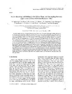
The RAMS forward and adjoint models were integrated with horizontal grid spacing of 6 km and 84 vertical levels using stretched height coordinate up to 17 km with a shortest step of 50 m and the largest 500 m. The horizontal grid step was chosen to be similar to the resolution of GOES observations (about 4 km, Table 1) but also affordable with the available computational resources. The horizontal grid step of 6 km in the cloudresolving model is only marginally cloud-resolving (Khairoutdinov and Randall, 2003) but serves the purpose in the current study to explore information content of the IR imager observations relative to the bulk 3D cloud distribution. The validity of the selected model configuration is demonstrated in comparison of data assimilation results to the GOES IR and radar reflectance observations in section 5. The RAMS initial and lateral boundary conditions were obtained from the operational regional Eta weather analysis archive at NCEP. The forecast model was first integrated for 15 hours starting at 00 UTC of March 21 2000. The data assimilation was performed within 11-14 UTC period using the original forecast as the first guess. The experiments were performed in two sets (Table 2). The first set (EXP1-EXP6) was designed to analyze information content of the observations and modeled background. In the second set (EXP7-EXP10) the sensitivity of the assimilation results to parameters in the assimilation procedure was investigated. Two assimilation windows of 1 hour duration were used for the experiments (11-12 and 13-14 UTC) except in EXP10 in which the 1 hour assimilation was cycled over 3 hour window (11-14 UTC). The observed atmosphere within J domain shown in Figure 1 is cloudy during the entire period (Figures 2 and 3). High ice clouds are present in the 11-12 UTC window evident in cold brightness temperatures in channels 4 and 5 in Figure 2 . The ice clouds
12
dissipate in the west half of the domain in the later period (13-14 UTC, Figure 3).
In the
model first guess simulation (i.e. without the assimilation) the cirrus cloud deck of small optical thickness is present in the 11-12 UTC period but dissipates entirely by 13 UTC. The brightness temperatures based on the model guess atmosphere in channels 4 and 5 are more than 30 K warmer in domain average than the observed even in the presence of thin cirrus in the 11-12 UTC period (Figure 5 a and e for channels 4 and 5, respectively). The significant differences in observed and modeled brightness temperatures and the associated cloud fields provided good basis for study of the value added by the assimilation.
4. Method of analysis
To facilitate the understanding of the information content of the observations and to evaluate the skill of assimilation and its sensitivity to key parameters in the data assimilation technique the experiment results were analyzed in 5 different measures. These are: 1) Cost function, 2) 2D brightness temperature distribution, 3) Domain error statistics in brightness temperature, 4) atmospheric temperature and humidity vertical sounding in selected points, and, 5) cloud radar reflectivity time series at a point The cost function measure is used to verify convergence of each data assimilation experiment and relative accuracy of different experiments when the cost function definition is the same. The brightness temperature 2D distribution is used to identify the observed cloud patterns and to evaluate the assimilation skill in terms of spatial and temporal variability. The domain errors are defined for the brightness temperatures as
13
point to point differences between the model and observations. A set of statistical parameters is then derived from the errors. The parameters are: mean, median, root mean square, standard deviation and empirical pdf. The domain error statistics provide both the compact analysis of quality of the specific assimilation result and a crude estimate of posterior errors in the observation space. The analysis of the cloud environment in the model before and after assimilation was performed by comparison of the vertical soundings of temperature and water vapor mixing ratio between different experiments and against the ARM observations at two locations labeled CF and B4 in Figure 1. The CF location is included in the assimilation domain, while the B4 facility is located at the edge of the outer-most model domain in the inflow region. The latter location is not influenced by the assimilation and serves the purpose of estimating errors in the lateral boundary condition. In the CF location the observed cloud radar reflectivity was used for independent verification of the assimilation results with respect to the vertical extent of clouds and the cloud type.
5. Information content of observations and model
The experiment results are summarized separately for the first and second period because they differ significantly in the observed and modeled cloud evolution.
14
5.1 Cloud information, first period
The data assimilation successfully converged in all experiments with channels 4 and 5 in the first set in the period 11-12 UTC (EXP1-EXP4).
In all experiments in this group the cost
function reduction is slow after about 8-9 iterations with only few percent change in last 5 iterations (Figure 4). As the reduction of cost function is slow, the analysis taken as an approximation to the optimal (minimum) solution. The overall reduction of cost function is one order of magnitude or larger. The final amplitudes are similar between the experiments in this set but cannot be compared directly because the cost function is defined by different BT data (i.e., different channels and observation frequency was used). Inspection of the cost function for individual observation times indicates that the minimum was achieved in the middle of interval, as expected for the 4DVAR data assimilation with the initial condition control parameter. In all experiments in the set EXP1-EXP4 the brightness temperatures at the end of assimilation shown in Figure 5 (b, c, d and f, g, h for the channels 4 and 5, respectively ) are significantly colder, have much smaller errors with respect to the observations (Figure 2 b and d) and more spatial variability than the guess (Figure 5 a and e). The individual grid point values of BT are different, however, for different experiments, so are the domain mean error amplitudes. Most importantly, it is evident in the results in Figure 5 that there is progression from less to more successful assimilation as more observational constraint is added. The least successful assimilation result was produced in the individual channel experiments (EXP1 and EXP2) with 30 minute observation frequency (Figure 5 b and f). The best result was achieved when all available observations from the channels 4 and 5 were assimilated together at 15 minute frequency (EXP4, Figure 5d and h). The experiment with both channels but 30 minute frequency produced the intermediate result (EXP3). The differences between assimilation results with the individual channels 4 and 5 (EXP1 and EXP2) and the improved assimilation when these
15
channels are combined in EXP3 and EXP4 suggest that they contain different information in the assimilation although the observed BTs are almost identical (compare Figures 2a with 2c and 2b with 2d). The different influence of channels 4 and 5 is discussed in the next section.
The domain error statistics in Figure 6 further demonstrate that the stronger observational constraint produces better assimilation results. The error distribution progresses from less to more Gaussian and from wider to narrower as the number of observations increases. The best observational constraint in EXP4 produces nearly zero domain mean error in the channel 4 (0.35 K) and small standard deviation (6.0 K) around the mean (Figure 6d and Table 3), while the channel 5 errors converged to small positive domain mean error (3.5 K) with similar standard deviation (Figure 6h and Table 3). Because of the single case sample the slightly better posterior domain mean error in channel 4 is not readily interpretable. The error statistics in EXP3 and EXP4 in Figure 6 show that the observations at different times contain independent information which is maximized in EXP4. The assimilation of channels 4 and 5 in EXP4 results also in the good vertical distribution of the ice cloud content and its evolution over the short period, evidenced in the comparison to the observed cloud radar reflectance at the ARM CF location in Figure 7. The improved vertical distribution of the ice cloud content shows that the information from the 2D BT observations is successfully extended into the 3D spatial domain due to the 4D dynamical correlations in the model. It is evident in Figure 7 that the observed low level liquid cloud is not simulated neither in the model guess nor in the assimilation. The absence of the low cloud in the model is the consequence of dry model troposphere below 4 km (Figure 8 a) which cannot be corrected with the channel 4 and 5 observations in the presence of the thick high clouds. 16
5.2 Humidity information, first period
The apparent cold BT bias in the channel 5 alone experiment (EXP2, Figures 5f and 6 f ) relative to the observations (Figure 2d) and the channel 4 experiment (EXP1, Figures 5b and 6b) is attributed to an overbuild of optically thick ice clouds in the southern and central portion of the domain (Figure 5f). The tendency for overestimation of the thick clouds in EXP2 could be partially explained by the sensitivity to water vapor. The sensitivity of BT to water vapor in the channels 4 and 5 is negative (i.e., more humidity results in lower BT) but is larger for the channel 5 (Greenwald and Christopher, 2000). This condition implies that for the same initial correction in temperature and cloud mixing ratio the water vapor in the model initial condition within the free troposphere would increase more in EXP2 than in EXP1. The more availability of the water vapor would then support the stronger build up of the high clouds in the latter experiment. The impact of different sensitivity to water vapor between the two channels also shows in comparison with the ARM sounding at the CF location. In Figure 8 (a and b) the guess forecast is dry throughout the column relative to the observed sounding. The assimilation of channel 5 alone increased the water vapor two times more than the channel 4 alone assimilation within 2.5-4.5 km layer (Figure 8b). This result suggests higher availability of the water vapor for conversion by lifting into the cloud mixing ratio above 5 km in EXP2. The increased lifting is apparent in vertical velocity data from the assimilation for all experiments (not shown). The change of domain mean BT error throughout the assimilation in EXP4 (Figure 9 ) shows that the assimilation has tendency
17
to overbuild the clouds everywhere in the first few iterations which is then corrected under the influence of observation’s spatial variability in subsequent iterations. The refinement of the cloud optical thickness after few initial iterations is not pronounced in the individual channel experiments because there are fewer observations. The vertical profiles of temperature and the corresponding temperature errors in the CF location in Figure 8 (c and d) show that the model atmosphere cools around 6-9 km in EXP1 and EXP2. This suggests that the conditions for the conversion of vapor into cloud are favorable in the adjustment to the observations. The cooling is slightly stronger in the channel 5 alone experiment. The temperature error is reduced where the cooling took place (Figure 8d). The absolute error reduction of both the temperature and humidity in Figure 8 is small but the sign and vertical distribution is consistent between the experiments, including EXP3 and EXP4 (not shown). Adding the water vapor channel (the channel 3) to channels 4 and 5 in EXP5 dos not improve the assimilation. The thick ice cloud is produced under the influence of channels 4 and 5, similar to the result in EXP4, but the model BT in channel 3 remains 14 K colder than the observed, which is already cold at around 220 K. Because the observed BT indicates the IR emission from above the cloud tops at around 10 km and the cost function sensitivity in the channel 3 peaks around the same altitude, relatively large perturbations are generated in the humidity and temperature initial condition around the tropopause.. The noisy perturbations at this level caused strong spurious gravity wave response in the model and unstable numerical solution in iteration 9 after the thick ice cloud was already developed, similar to EXP4. This result implies that after the minimum is nearly reached in the cost function convergence under the influence of dominant
18
observations, in this case the channels 4 and 5 which are sensitive to the clouds, the remaining iterations generate noise which could cause numerical instability in the model.
5.3 Cloud triggering, second period
The role of sensitivity to humidity in the channel 5 is shown more explicitly in the experiment for the second period (13-14 UTC, EXP6). In EXP6 the model first guess is cloud free everywhere while the observations display dissipating ice clouds (Figure 3). The guess cost function in EXP6 is larger and also converges to significantly higher value than in the first period (Figure 2, compare curves EXP4 and EXP6). The convergence was achieved in only few iterations. The cost function reaches minimum in time at the end of interval, rather than in the middle as in EXP1-EXP4. Starting from no clouds in the guess forecast the model developed thick ice clouds in the north-east and partially in the south-east parts of the domain and thin or no clouds in the central and south-west regions early in the period. These features were then advected in a northeasterly direction in the second portion of the period with some dissipation in the north-west corner. Figure 10 shows BT at the end of assimilation period (panels a and c for the channels 4 and 5, respectively). The model clouds are made entirely of the pristine ice and snow hydrometeors indicating that the ice cloud formation is favored. The extreme cold and warm pattern in the model cloudiness results in the domain average mean error in BT of only 2.3 K and –0.2 K, in the channels 4 and 5 respectively, at the end of assimilation period (Table 3 and Figure 10 b and d), but do not compare well with the observed pattern (Figure 3 c and d). The domain error statistics in
19
Figure 10 (c and d) also show non Gaussian distribution of the final analysis errors with extreme tails, unlike for the experiments in the first period. The cloud initiation in the early stage of assimilation occurred in the assimilation in regions where there were colder observed BT and where the sensitivity to water vapor in channel 5, the lifting and the cooling were strong enough to trigger cloud formation at levels above 5 km. The model lower troposphere remained dry in the assimilation as in the experiments from the first period. The ice cloud formation mechanism could not produce a correct observed evolution because the IR imager observations do not contain explicit information about vertical variability of the cloud environment while the model cloud first guess and lateral boundary conditions contained large errors. The dry advection from the lateral boundaries was confirmed by comparing the model and observed humidity sounding for the ARM B4 location. With the poor first guess, the limitation in EXP6 assimilation appears to be in the sensitivity produced with the adjoint computation. The adjoint computation in VISIROO produces zero sensitivity to the cloud parameters for the first guess that is cloud free which then forces the assimilation to initially relay on the adjustment through the humidity and temperature fields. Because these fields are not well constrained with the IR observations in the presence of high clouds the assimilation results are not very good. It could be argued that the problem of limited local sensitivity in the assimilation may be reduced by broadening exploration of the model sensitivities around the given guess as done, for example, in ensemble based data assimilation techniques (van Leeuwen, 2001). Application of the ensemble techniques in the CRM satellite data assimilation is a possibility, but given large number of probable states which could satisfy the limited
20
observational constraint, an optimally more accurate solution is only possible by adding observations that would more uniquely constrain the cloud triggering. For example, the additional observations should have high information content about mesoscale distribution of temperature and humidity and possibly the cloud condensation nuclei. The 4DVAR data assimilation technique is capable of accurate representation of the sensitivity to the quantities with more continuous spatial distributions than the cloud hydrometeors. The recent study by Lee and Lee (2003) specifically demonstrated the benefit of assimilating the water vapor and temperature observations in triggering a heavy precipitation event using the 4DVAR data assimilation technique with a mesoscale model. In the current study the additional satellite observations were not used because they would require development of additional components in the RAMDAS observational operator, which will be addressed in future studies. Currently, a potential for improving the model atmosphere to support formation and maintenance of the ice clouds in 13-14 UTC period is addressed in a limited way by using the sequence of 3 1hour assimilation cycles starting at 11 UTC (EXP10) when the model first guess contains the thin ice cloud. The results of EXP10 are discussed in section 6.3.
21
6. Sensitivity to assimilation parameters
6. 1 Sensitivity to model error There is very little experience about the systematic model errors in the CRMs with respect to the satellite remote sensing observations because they are typically not verified against these observations. The lack of specific experience requires the use of simple specification of the model error derived from the synoptic scale data assimilation applications in NWP such as in Zupanski et al (2002) and Lee and Lee (2003) and testing of the impact of this approach in the CRM data assimilation for the selected cases. In EXP7 and EXP8 the model error was specified as linear temporal bias over short assimilation period of 1 hour with the spatial variance and decorrelation length the same as for the initial condition errors (Table 2). In the 11-12 UTC period with all available observation times, the final assimilation result (EXP4) is already very good without the model error. The effect of adding the model error in EXP4 was surprising. The linear forcing term in the nonlinear governing equations generated a perturbation in the model that caused an unstable nonlinear model solution at the third iteration and no convergence of the data assimilation. To test the influence of model error in a manner more similar to the previous experience in NWP with less observational constraint, the experiment was repeated but using EXP1 design: the channel 4 only with 30 minute observation frequency. The cost function is reduced almost an order of magnitude in only 3 iterations, much faster than in EXP1, but it does not change much after that (Figure 4, curve EXP7A). The converged assimilation with the model error shows that the linear error forcing could be used to reduce more quickly the model domain wide bias when there are fewer
22
observations but the refinement of spatial variability that is better constrained with more observations is not well modeled with this approach. In the second period (EXP9) the model error was added to EXP6, where the first guess error was obviously large in the cloud fields. The effect was similar as for the first period. The convergence was not achieved due to the unstable solution in the nonlinear model. It is beyond the scope of this study to fully address the modeling of model error in CRMs. The current results indicate that: a) The 4DVAR data assimilation with the model error in the form of linear forcing in the CRM causes unstable model solutions when the adjustment in the model occurs at small spatial scales and b) The current model error specification cannot compensate for the gross errors resulting from the lack of constraint by observations with respect to cloud environment and under the circumstances of large lateral boundary condition errors. A more effective modeling of the model errors in CRMs may need to include estimation of model parameters within the data assimilation framework.
6.2 Sensitivity to background error correlation scale
The preliminary experiments not included in Table 2 with the horizontal decorrelation length of 50 km produced the BT distribution and amplitudes similar to EXP1-EXP4 results but smoother. The decorrelation length was then reduced to 30 km. In EXP4 this change resulted in spatial variability similar to the observed BT with the exception of small scale features at the scales of about 15 km (for example, compare Figure 5d with 2b). To test whether the smaller scale features could be captured the
23
decorrelation scale was reduced to 15 km in EXP9. The result was somewhat unexpected. Instead of increased spatial variability the final brightness temperatures are characterized with a large scale cold region surrounded by warmer regions near the inflow lateral boundaries (Figure 11a). The spatial variability within this pattern is slightly higher than in EXP4 but the dominant feature is of the large scale. The domain mean BT error is almost -10 K with large standard deviation of about 11 K and non Gaussian distribution (Figure 11b). The dominance of large scale pattern in BT errors could be explained by considering resolvable spatial scales in the model. The model horizontal grid spacing of ∆x = 6 km determines that the smallest resolvable scales are about 25-30 km as
consequence of horizontal numerical diffusion (Pielke, 2002). The initial condition error decorrelation length of 15 km is thus below the dynamical resolution of the model. This condition causes that the projection of cost function sensitivity from the adjoint model solution at 2 ∆x ≈ 15 km in the initial condition update in the optimization algorithm, is alliased to longer scales which apparently favors the tendency toward building a slightly thicker ice cloud over larger domain and consequently colder BT.
6.3 Sensitivity to first guess
The cycling of the data assimilation in EXP10 produced a better first guess in the period after 12 UTC and a better BT result at 14 UTC. The expected lateral boundary conditions error influence is apparent in Figure 12, but the final BT result was better than in EXP6 in which the first guess at 13 UTC is the original model simulation without the
24
assimilation. In EXP10 the large scale cold and warm pattern of BT (Figure 12) is similar to the observed (Figure 3b), but the amplitudes are larger in both signs. Most of the region with warm BT is cloud free due to the lateral boundary influence. These results show that the data assimilation cycling would improve the model first guess in the assimilation but the benefit is limited by the lateral boundary condition errors in small domains. In the current 4DVAR data assimilation systems with limited area models including RAMDAS the lateral boundary condition errors are folded into the model error control vector space. Zupanski (1997), Zupanski et al. (2002) and Lee and Lee (2003) demostrate benefits of this approach in applications with synoptic scale assimilation of non-satellite measurements in domains significantly larger than the domain used in this study. It is shown in section 6.1 that the linear model error specification is not suitable for the CRM data assimilation with the high spatial resolution satellite observations. The results suggest that the lateral boundary condition errors in the assimilation should be separated from the remaining model error. Devising a new algorithm to incorporate this approach is beyond the scope of the current study and will be addressed in the future.
7. Summary and conclusions
This study addresses the problem of 4D estimation of cloudy atmosphere on cloud resolving scales using assimilation of the satellite observations. The motivation is to develop methodology for accurate representation of 4D cloud properties and the atmospheric environment on cloud resolving scales. The problem is approached initially
25
by assimilation of the GOES imager observations into the cloud resolving model. It is well known that the GOES and other imager observations are excellent source of cloud data because of their spectral characteristics and good spatial and temporal resolution but these data are not yet considered in the current data assimilation systems. In this study the new 4DVAR research data assimilation system was applied to analyze the information content of the GOES imager IR channels relative to the modeled bulk cloud properties and the atmospheric environment for the case of non-precipitating and non-convective multi-layered cloud evolution. The sensitivity to key parameters in the data assimilation system and verification of the assimilation results against independent observations of the clouds and their environment was also addressed. The main conclusions are •
The spatial distribution of the modeled ice cloud mass is significantly improved
in 4D by the assimilation of IR window channels ( 10.7 µ and 12.0µ wavelengths) with
15 minute frequency when the model already contains conditions for the ice cloud formation. The assimilated cloud in this case is in good agreement with the independent cloud radar measurements at the ARM central facility. This result implies that the CRM representation of 4D distribution of the hydrometeor mass could be systematically improved by assimilation of the high spatial and temporal resolution geostationary satellite measurements. • The assimilation results clearly demonstrate that increasing the observational
constraint from individual to combined window measurements and from less to more frequent observation times systematically improves the assimilation results.
26
• The model temperature and humidity profiles improve only slightly in response to
the IR window observations and relative to independent single point atmospheric sounding observation at the ARM central facility, but the improvement is dynamically consistent with the cloud improvement. • The assimilation of the upper tropospheric water vapor channel does not
contribute to improvements in the assimilation in the presence of thick ice clouds. • The channel 4 and 5 measurements exhibit independent contribution in the
assimilation because the results improve with combining the channels. The known higher sensitivity of the channel 5 to water vapor contributes more to positive change in the modeled humidity. • The assimilation of the GOES imager window channels is unable to help generate
low level liquid cloud in the model below the ice cloud because the observations are not sensitive to the low cloud in the presence of high clouds above. The additional observations of the lower troposphere are needed to address this problem. • Similarly, the imager IR window channels do not provide sufficient constraint to
address the cloud triggering conditions. Other remote sensing observations must be used. • Advection of a cloud free atmosphere from the lateral boundaries in the regional
model simulations causes significant error in the cloud forecast and the associated assimilation. This points to the general problem of downscaling in small regions from the global or larger domain size atmospheric analysis. This problem is partially solved by assimilation of regional satellite observations within a domain several times smaller than the model simulation domain but large enough to capture the cloud evolution.
27
• The instability of assimilation results with the linear model error suggest that the
current specification of the model error in RAMDAS that was adopted from other data assimilation studies in the Numerical Weather Prediction applications is not suitable for the cloud resolving data assimilation. • The horizontal decorrelation length scale of 15 km which is compatible with
spatial variability in the observed brightness temperatures in the study case produced inferior assimilation result to the experiments with the decorrelation length of 30 km. This is the consequence of spatial discretization in the modeled dynamics which controls effective horizontal spatial scales, typically larger than 4 times the model horizontal grid spacing. The effective horizontal scales in the current study are about 25-30 km, for the model grid of dx = 6 km. The result implies that to take advantage of the full resolution in GOES imager observations the model in the data assimilation should be integrated with resolution several times finer than the observations’ native resolution. In summary, the current experience with the cloud resolving data assimilation using the GOES imager IR observations suggests a strong potential for improving the 4D cloud analysis using the high resolution satellite remote sensing with explicit cloud models but this complex problem requires further research. The new research should address use of other satellite observations with additional information content to constrain the cloud triggering conditions, higher resolution modeling and an in-depth study of model errors.
Acknowledgments This study was supported by the DoD Center for Geosciences/Atmospheric Research at Colorado State University under the Cooperative Agreement (#DAAL01-98-2-0078) with the Army Research Laboratory.
28
References
Atlas, D., 1990: Radar in Meteorology. American Meteorological Society. pp 860. Benedetti, A., T. Vukicevic, and, G. L. Stephens, 2003: Varaitional assimilation of radar reflectivities in a cirrus model. II: Optimal initialization and model bias estimation. Quart. J. Roy. Meteorol. Soc., 129, 301-319. Bennett, F., A., 2002: Inverse Modeling of the Ocean and Atmosphere. Cambridge University Press. Chevallier, F., and, G. Kelly, 2002: Model Clouds as Seen from Space: Comparison with Geostationary Imagery in the 11- m Window Channel. Mon. Weath. Rev., 130, 712–722. Cohn, S. E., 1997: An introduction to estimation theory. J. Meteor. Soc. Japan, 75, 257-288. Cotton, W.R., R.A. Pielke Sr., R.L. Walko, G.E. Liston, C. Tremback, H. Jiang, R.L. McAnelly, J.Y. Harrington, M.E. Nicholls, G.G. Carrio, and J.P. McFadden, 2003: RAMS 2001: Current status and future directions. Meteor. Atmos. Phys., 82, 5-29. Deeter, M., and K. F. Evans, 1998: A hybrid Eddington-single scattering radiative transfer model for computing radiances from thermally emitting atmospheres. J. Quant. Spect. Rad. Transfer, 60, 635-648. Derber, J., C., and, W.-S., Wu, 1998: The use of TOVS cloud-clear radiances in the NCEP SSI analysis system. Mon. Wea. Rev., 126, 2287-2302. Enting, J., 2002: Inverse Problems in Atmospheric Constituent Transport. Cambridge Atmospheric and Space Science Series.
Evans, K. F., 1998: The Spherical Harmonics Discrete Ordinate Method for Three-Dimensional Atmospheric Radiative Transfer, J. Atmos. Sci., 55, 429-446.
29
Greenwald, T. J., and, S. A, Christopher, 2000: The GOES I-M Imagers: new tools for studying microphysical properties of boundary layer stratiform clouds. Bull. Amer. Meteor. Soc., 81, 2607-2620.
Greenwald, T. J., T. Vukicevic, and, L. D. Grasso, 2004: Adjoint sensitivity analysis of an observational operator for cloudy visible and infrared radiance assimilation. Q. J. R. Met. Soc. 130, 685-705. Greenwald, T. J., R. Hertenstein, and T. Vukicevic, 2002: An all-weather observational operator for radiance data assimilation with mesoscale forecast models. Mon. Wea. Rev., 130, 1882-1897. Guyot, A., J. Testud, and T. P. Ackerman, 1999: Determination of the radiative properties of stratiform clouds from a nadir-looking 95-GHz radar. J. Atmos. Ocean. Sci., 17, 38-50. Kidder, S. Q., and, T. H. Vonder Haar, 1995: Satellite meteorology: An introduction. Academic Press Inc., pp 466. Khairoutdinnov, M. F., and, D. A. Randal, 2003: Cloud resolving modeling of the ARM Summer 1997 IOP: Model formulation, results, uncertainties and sensitivities. J. Atmos. Sci., 60, 607-624. Kummerow, C., W. S. Olson, and L. Giglio, 1996: A simplified scheme for obtaining precipitation and vertical hydrometeor profiles from passive microwave sensors. IEEE Tran. Geosci. Remote. Sens., 34, 1213-1232. Lee, M.-S., and, D.-K., Lee, 2003: An application of weekly constrained 4DVAR to satellite data assimilation and heavy rainfall simulation. Mon. Wea. Rev., 131, 2151-2165. McMillin, L. M., L. J. Crone, M. D. Goldberg, and T. J. Kleespies, 1995: Atmospheric transmittance of an absorbing gas, 4. OPTRAN: A computationally fast and accurate
30
transmittance model for absorbing gases with fixed and variable mixing ratios at variable viewing angles, Appl. Opt., 34, 6269-6274. Parrish, D., F., and, J., C., Derber, 1992: The National meteorological Center’s spectral statistical interpolation analysis system. Mon. Wea. Rev, 120, 1747-11763. Pielke, R. Sr., 2002: Mesoscale Meteorological Modeling. Academic Press, A Division of Harcourt, Inc., pp 676. Rossow, W. B., and A. Schiffer, 1999: Advances in understanding clouds from ISCCP. Bull. Amer. Meteor. Soc., 80, 2261-2287. --------, and L. C. Garder, 1993: Coud detection using satellite measurements of infrared and visible radiances for ISCCP. J. Climate, 6, 2341-2369. Snyder, C., and, F., Zhang, 2003: Assimilation of Simulated Doppler Radar Observations with an Ensemble Kalman Filter. Mon. Wea. Rev, 131, 1663–1677. Sun, J., and., N. A. Crook, 1998: Dynamical and microphysical retrieval from Doppler radar observations using a cloud model and its adjoint. Part II: Retrieval experiments of an observed Florida convective storm. J. Atmos. Sci., 55, 835-852. Stephens, G. L., 2002: The CloudSat mission and the A-Train. Bull. Amer. Meteor. Soc., 83, 1771-1790. Stokes, G. M., and, S. E. Schwartz, 1994: The Atmospheric radiation Measurement (ARM) Program: Programmatic background and design of the cloud and radiation test bed. Bull. Amer. Meteor.l Soc., 75, 1201-1222. Tarantola, A., 1987: Inverse Problem theory: Methods for data fitting and model parameter estimation. Elsevier. van Leeuwen, 2001: An Ensemble Smoother with Error Estimates. Mon. Wea. Rev . 129, 709– 728.
31
Vukicevic, T., R. Braswell, and, D. Schimel, 2001: A diagnostic Study of temperature controls on global terrestrial carbon exchange. Tellus, 53B, 150-170. Vukicevic, T., T, Greenwald, M. Zupanski, D. Zupanski, T. Vonder Haar, and, A. Jones, 2004: Mesoscale cloud state estimation from visible and infrared satellite radiances. Mon. Wea. Rev. , 132, 3066-3077. Wu, B., J. Verlinde, and, J. Sun, 1999: Dynamical and microphysical retrievals from Doppler radar observations of a deep convective cloud. J. Atmos. Sci., 57, 262-283. Zhang, F., C., Snyder, and, J. Sun, 2004: Impacts of Initial Estimate and Observation Availability on Convective-Scale Data Assimilation with an Ensemble Kalman Filter. Mon. Wea. Rev., 132, 1238–1253. Zupanski, D., 1997: A general weak constraint applicable to operational 4DVAR data assimilation system. Mon. Wea. Rev., 125, 2274-2292. Zupanski, M., D., Zupanski, D. Parrish, E., Rogers, and, D. DiMego, 2002: Four-dimensional variational data assimilation for the blizzard of 2000. Mon. Wea. Rev., 130, 1967-1988. Zupanski, M., D. Zupanski, T. Vukicevic, K. Eis, and, T. Vonder Haar, 2005: CIRA/CSU Fourdimensional variational data assimilation system. Mon. Wea. Rev. Accepted, to appear in April 2005.
32
Figure captions
Figure 1: Integration domains: F- forward model and adjoint simulation domain, A –
data assimilation sub-domain and J – cost function sub-domain. CF and B4 mark locations of the ARM central and extended facilities, respectively.
Figure 2: Observed GOES imager brightness temperatures in K within sub-domain S in
Figure 1 for the period 11-12 UTC March 21 2000: a and c are for 11:30 and b and d for 12:00 Left column is for the channel 4 and right for the channel 5.
Figure 3: Observed GOES imager brightness temperatures in K within S domain in
Figure 1 for the period 13-14 UTC March 21 2000: a and c are for 13:30 and b and d for 14:00. Left column is for the channel 4 and right for the channel 5.
Figure 4: Cost function J as function of iteration for various experiments. The
experiments are outlined in Table 2. The cost function is normalized with values at zero iteration for each experiment (i.e., the model guess).
Figure 5: Brightness temperatures (BT) after assimilation in units of K for channels 4
and 5, left and right column, respectively, within S domain shown in Figure 1, valid at 12 UTC: (a) and (e) show the model guess, (b) is for EXP1, (f) is for EXP2, (c) and (g) are for EXP2 and (d) and (h) are for EXP4.
33
Figure 6: Brightness temperature error frequency after assimilation for channels 4 and 5,
left and right column, respectively, within S domain shown in Figure 1. The error sample is defined as point by point difference between model and observation within S domain. (a) and (e) show the model guess, (b) is for EXP1, (f) is for EXP2, (c) and (g) are for EXP2 and (d) and (h) are for EXP4.
Figure 7: Cloud radar reflectivity as function of time at the ARM CF location: (a)
observed, (b) model after assimilation in EXP4 and (c) model guess.
Figure 8: Vertical atmospheric sounding at the ARM Central facility location, observed
and modeled: (a) vapor mixing ratio, (b) temperature, (c) vapor mixing ratio error and (d) temperature error. The error is defined as model minus observed. The units are gkg −1 and K for the water vapor mixing ratio and temperature, respectively.
Figure 9: Domain brightness temperature error statistics as function of iteration for: (a)
channel 4 and (b) channel 5 in EXP4.
Figure 10: Model brightness temperatures (BT) in K after the assimilation of channels 4
and 5 for the period 13-14 UTC in EXP6 and the associated domain error statistics. a) channel 4 BT, (b) channel 5 BT, (c) BT error frequency for channel 4, and (d) BT error frequency for channel 5.
34
Figure 11: (a) Model brightness temperature in K at the end of assimilation in EXP9 and
(b) the associated domain error statistics.
Figure 12: (a) Model brightness temperature in K at the end of assimilation in EXP10
(14 UTC).
35
Table captions
Table 1: Characteristics of the GOES imager channels Table 2: Characteristics of the data assimilation experiments Table 3: Error statistics in the data assimilation experiments
36
Table 1: Characteristics of the GOES I-M imagers (after Greenwald and Christopher, 2000).
Channel 1 2 3 4 5
Wavelength range (µm) 0.52-0.74 3.79-4.04 6.47-7.06 10.2-11.2 11.6-12.5
Effective spatial resolution (km × km) 0.57 × 1 2.3 × 4 4×8 2.3 × 4 2.3 × 4
Precision specs (*% albedo or K at 300 K) 0.20* 0.23 0.22 0.14 0.26
Description Visible Near-infrared IR water vapor IR window IR window/water vapor
37
Table 2: Experiment characteristics
Experiment
Data assimilation interval (UTC on March 21 2000)
Assimilated channels
Observation frequency (minutes)
EXP1 EXP2 EXP3 EXP4 EXP5 EXP6 EXP7 EXP7A EXP8 EXP9 EXP10
11-12 11-12 11-12 11-12 11-12 13-14 11-12 11-12 13-14 11-12 11-14
4 5 4, 5 4, 5 3, 4, 5 4, 5 4, 5 4, 5 4, 5 4, 5 4, 5
30 30 30 15 15 15 15 30 15 15 30
Horizontal background decorrelation length, Lh (km) 30 30 30 30 30 30 30 30 30 15 30
38
Model error no no no no no no yes yes yes no no
Table 3: Brightness temperature domain error statistics in degrees K Experiment
Domain mean ch4/ch5
Guess EXP1 EXP2 EXP3 EXP4
31.3/36.6 -1.4/na na/-7.3 -4.3/-1.4 0.35/3.5
Standard deviation ch4/ch5 7.2/6.6 9.0/na na/9.8 8.9/9.1 6.0/5.8
EXP6 EXP9
-0.2/2.4 -9.9/-10.2
16.2/16.9 10.9/11.1
Median ch4/ch5
RMS ch4/ch5
29.9/35.5 -0.9/na na/-9.8 -4.8/-1.8 0.02/2.8
32.1/37.3 9.1/na na/12.1 9.9/9.3 6.0/6.7
0.4/2.4 -11.3/-12.4
16.2/17.0 14.7/15.2
39
37.7 N
CF
B4 J A
35.1 N F 99.3 W
96.0 W
Figure 1: Integration domains: F- forward model and adjoint simulation domain, A –
data assimilation sub-domain and J – cost function sub-domain. CF and B4 mark locations of the ARM central and extended facilities, respectively.
40
Figure 2: Observed GOES imager brightness temperatures in K within sub-domain S in
Figure 1 for the period 11-12 UTC March 21 2000: a and c are for 11:30 and b and d for 12:00 Left column is for the channel 4 and right for the channel 5.
41
Figure 3: Observed GOES imager brightness temperatures in K within S domain in
Figure 1 for the period 13-14 UTC March 21 2000: a and c are for 13:30 and b and d for 14:00. Left column is for the channel 4 and right for the channel 5.
42
Figure 4: Cost function J as function of iteration for various experiments. The
experiments are outlined in Table 2. The cost function is normalized with values at zero iteration for each experiment (i.e., the model guess).
43
Figure 5: Brightness temperatures (BT) after assimilation in units of K for channels 4
and 5, left and right column, respectively, within S domain shown in Figure 1, valid at 12 UTC: (a) and (e) show the model guess, (b) is for EXP1, (f) is for EXP2, (c) and (g) are for EXP2 and (d) and (h) are for EXP4.
44
Figure 6: Brightness temperature error frequency after assimilation for channels 4 and 5,
left and right column, respectively, within S domain shown in Figure 1. The error sample is defined as point by point difference between model and observation within S domain. (a) and (e) show the model guess, (b) is for EXP1, (f) is for EXP2, (c) and (g) are for EXP2 and (d) and (h) are for EXP4.
45
Figure 7: Cloud radar reflectance as function of time at the ARM CF location: (a)
observed, (b) model after assimilation in EXP4 and (c) model guess.
46
Figure 8: Vertical atmospheric sounding at the ARM Central facility location, observed
and modeled: (a) vapor mixing ratio, (b) temperature, (c) vapor mixing ratio error and (d) temperature error. The error is defined as model minus observed. The units are gkg −1 and K for the water vapor mixing ratio and temperature, respectively.
47
Figure 9: Domain brightness temperature error statistics as function of iteration for: (a)
channel 4 and (b) channel 5 in EXP4.
48
Figure 10: Model brightness temperatures (BT) in K after the assimilation of channels 4
and 5 for the period 13-14 UTC in EXP6 and the associated domain error statistics. a) channel 4 BT, (b) channel 5 BT, (c) BT error frequency for channel 4, and (d) BT error frequency for channel 5.
49
Figure 11: (a) Model brightness temperature in K at the end of assimilation in EXP9 and
(b) the associated domain error statistics.
50
Figure 12: (a) Model brightness temperature in K at the end of assimilation in EXP10
(14 UTC).
51