Jul 7, 2003 - I propose a new poverty measure, integrating the food content of poverty lines and ... Distribution System (PDS) on poverty and food security.
The Public Distribution System in India: Counting the poor from making the poor count Ahmed Tritah∗ GREMAQ, Universit´e des Sciences Sociales, Toulouse, France July 7, 2003
Abstract This paper investigates the effect of food subsidies on food security and poverty in India. Using propensity score matching methods I found that while the PDS has a poor record on reaching the poor, conditional on having access to PDS, the subsidy is entirely consumed. Moreover I found that food subsidies going through the PDS exert a multiplier effect on quantity consumed. This findings point to a reevaluation of the impact of PDS with respect to its main objective which is food security. I propose a new poverty measure, integrating the food content of poverty lines and shows that relative to this poverty line PDS has benefited the poor. ∗
I thank the World Bank Economic Development Research Group, for its hospitality during the winter 2003 and for providing me with the data, and in particular Klaus Deininger and Dina Umali Deininger from South Asia Rural Development Sector, for giving me the opportunity to undertake this research. The usual disclaimer apply.
1
1
Introduction
Over the past decade a series of events in India have brought the question of food security into sharp focus (UNDP 1999). According to the Food and Agricultural Organization , India alone accounts for over 400 million poor and hungry people. For a nation long inured to scarcity and starvation the problem is ironic: it is the one of plenty. Why in a food surplus nation where buffer stock are three time what is required for food security, thousands still die of malnutrition and hunger? While the objective of food security has been reached, the fundamental individual right for food has not. The purpose of the present research is to evaluate the impact of the Indian Public Distribution System (PDS) on poverty and food security. The results are of immediate policy interest with respect to the current debate and re-shaping of the Indian Public Distribution System. Of all the safety net operations that exist in India, the most fare reaching in terms of coverage as well as public expenditure on subsidy is the PDS. PDS provides rationed amounts of basic food items (rice, wheat, sugar, edible oils) and other non food products (kerosene, coal, standard cloth) at below market prices to consumers through a network of fair price shops disseminated over the country. While measurement of poverty is a heated issue in India (Deaton 1999, Deaton and al. 2000) to the best of my knowledge only one study has quantitatively evaluated the extend to which PDS alleviate poverty (Rafhakishna and al, 1997). The PDS had been criticized for its urban bias and its failure to serve effectively the poorer sections of the population. As main of studies on benefit incidence of fiscal transfer, this evaluation of PDS failed to consider the counterfactual and take the fiscal 2
transfer as the net gain accruing to the poor using PDS. My claim here is that recent advances in program impact literature provide powerful tools to evaluate the benefit incidence of fiscal transfer through food subsidy on food security and poverty. The power of these method is that by controlling for selection into the program the implicitly take into account behavioral heterogeneity and estimate the impact net of this heterogeneity. Since June 1997 PDS turned into the Targeted Public Distribution System, the aim is to target the poorest household by differentiating the access quantities and prices at which one is allow to buy. The differentiation is made with respect to the state official poverty lines. Those households below the poverty line (BPL households) are entitled with ration card that allows them to buy more quantity at a higher subsidized price. The main issue of TPDS is that as any targeting program it will always involve, albeit to different degree, problems of imperfect targeting. That is the system is likely to include people that should be excluded and exclude household that should be included. However targeting for food is somewhat more problematic because it deals with contingencies that one can not perfectly foreseen. In particular you may not need the government aid today but tomorrow if your income fell you will need it. Hence it is not clear given this contingencies how one should design a system targeting to those in need at every time. One way to do that is to introduce the concept of self-selection. That is to say that the program is designed in such a way that those who are not targeting have no incentive to go into the program. This paper estimates the expenditure gains and the reduction in poverty if any that is attributable to the TPDS. For this purpose I apply recent
3
advances in propensity score matching methods (PSM) (Rosenbaum and Rubin, 1983; Heckman et al, 1997, 1998). These methods allow us to draw a statistical comparison group to TPDS users from the same survey. Matching methods have been quite widely used in evaluations. However matching on propensity score rather than arbitrarily set of characteristics is the optimal method and have received a renewed interest since the seminal paper of Rosenbaum and Rubin, 1983. A number of feature to TPDS make it suitable for PSM methods. Other evaluation methods requires randomization or a baseline and this is not available here since the program has a nation wide coverage1 . TPDS has large impact in the Indian economy, what we are doing here is a partial equilibrium analysis, I will just consider the impact of fair price shops on poverty assuming away any general equilibrium effect on prices and quantities due to TPDS. However one should bear in mind that Food Corporation of India has as much as three times the necessary quantities needed to insure food security, and no doubt that by insuring a minimum price to producer it has impact on open market prices that can not be evaluated without using a general equilibrium approach. Studies have show that PDS has pushed private prices upward (Dumali and al 2001). Hence any feasible evaluation method need to be considered as an upper bound of the impact of PDS. An important advantage of PSM methods here is that the are suitable to studying the heterogeneity of program. This is of obvious interest here since 1 However I can identify a set of non TPDS users that have not used TPDS for exogenous reasons I can get ridd of bias due to selection into the program. This potential user can then form a control group along which the impact of the treatment is evaluated.
4
TPDS is precisely targeted toward the poor, one should observe a greater impact among the poor than others. Identity of beneficiaries are important for designing better policy and determine links between poverty and other characteristics that hamper or on the contrary favor better targeting. The following section discusses in more detailed the fiscal content of PDS. The methods for identifing the impact on poverty and food security of PDS are described in section 3. Section 4 present the data and primary descriptive statistics. Section 5 gives the impact estimates on poverty and food security? Section 6 concludes.
2
The Indian Public distribution system
2.1
The fiscal background
The rural Indian spend 64% of its budget on food. Food share is an inverse indicator of welfare2 (e.g. Deaton 1997): it follows that food security should be a major focus of policies concerned with well being in this society. In terms of both coverage and public expenditure, the most important food safety net is the Public Distribution System. Of the 200 million tones of food grains produced in 1999-2000, about 29 million where produced by the government under PDS, which now support the largest network of ”fair price shops” in the world.(458499 shops in 1999). These provides rice, wheat sugar, edible oil, soft cake and kerosene oil at subsidized prices. The PDS is managed by state governments. The central government based on the population state and its share of below poverty line households and above 2
The fooshare is remarkbly stable within the three first quitile of the income distribution around 75% it strated to decline at the fourth quintile...
5
poverty line households, determine the total procurement of food grains and total allocation across states. The government also determines the Central Issue Prices (CIP) for commodities. The state government then determines the off-take, the public delivery, and the list of commodities provided. The state government is allow to add to the CIP the transactions cost of keeping the stock and of delivering. Locations of the fair price shops are determined by the officials at the district level3 . There is enormous variation in the density of the fair price shops as also in the regularity of supplies both across and within states. The PDS took shape soon after the Bengal famine in 1943. It evolves in the 1950s and 1960s as a mechanism for providing price support to producers and at the same time as providing food subsidy for consumers. At that time the country was threatened by national-level food shortages and there was rapid food price inflation, especially in urban areas. By the 1980s, India had generated a surplus of foodgrains and the incidence on poverty had declined progressively for about 50 per cent in the 1960s to about 30 per cent in the 1990s. As a result the welfare component of the PDS gains strength in the 1980s , when it was considerably extended to rural and tribal blocks, with and explicit view to reaching areas of high poverty incidence. In the context of currency devaluation and economic reform in the 1990s, procurement and issue prices of PDS commodities were increased leading the government to mitigate the adverse welfare consequences by better targeting of PDS to the poor. Until 1992, there was universal entitlement to the PDS but it has since 3
Note that this raises a problem of three level targeting. The government first target quantities based on state poverty estimation. Then the state target the distribution of food to the local district, which in turn target the fairprice shops and quantities to the population. Every unit level make decision based on specific information for targeting which is in some extent private knowledge.
6
been restructured. In 1997 it was replaced by the Targeted PDS (TPDS).in which targeting was shifted from poor regions to poor households and the subsidy differential between the poor and non poor was widened. More specifically, 10kg of foodgrains were available at a highly subsidized price per family per month for families below the poverty line. Those classify as non poor get no subsidy though they are served by fair price shops, which can play a useful distributional function in areas where private shops have not emerged. The problem of crowding out effect may exist if the poor are credit constraint and if they rich are not. When asked the main reason why people have not used fair price shops is that because the commodities were not available in sufficient quantity or quality.
2.2
The evaluation problem
India is embarked on a program of economic reforms in 1991 with the objective of achieving macroeconomic stabilization and structural adjustment, the latter being closely tied to getting prices right. Both processes encourage government expenditure reduction and the removal of subsidies. In this context the PDS has commended considerable attention. It has been argued that it is an obsolescent and fiscally unsustainable institution.(e.g. Umali Deininger and Deininger 2001, World Bank 1998b). These authors have also argues that the PDS has a poor record on reaching the poor. Hence the move towards slimming the system and targeting the subsidy at the poor. This was done in June 1997, moving through a universal public distribution system toward a targeted public distribution system. There is still a debate on whether the PDS should be phase out and replaced with more effective instruments for reaching the poor. While the cost effectiveness of the sys7
tem has been put in scrutiny, we still lack a program evaluation impact of TPDS. For that we need to investigate the benefit incidence of TPDS that is (1) access of poor to foodgrains at subsidized price and (2) conditional on the access we need to evaluate the progresivity of the TPDS with regard to poverty. That is are the poor more likely tu use PDS than others? Conditional on access does the poor benefit more in absolute term than others?Conditional on access are the poor benefiting more than proportionately to their overall share of income or expenditure? To what extend are the impact translated into poverty variation figures4 ?. The poverty impact of TPDS is the difference between poverty level with the TPDS and the poverty level without it. The with data are observable while the ”without” data are fundamentally unobservable. This is the well known problem of causal inferences (Holland 1986). Common practice for assessing the distributional and poverty impact, the fiscal benefit incidence analysis, is straightforward but ignore the counterfactual taking the transfer as the net benefit accruing to household, ignoring any behavioral responses. Benefit incidence of PDS has two component the price and the quantity the overall being the product of both. Previous evaluation consider only the with and without the program effect on prices, but fail to consider the without effect on quantities. This is to assume that those affecting by PDS does not change their consumption behavior as the result of PDS. 4
Attention paid to poverty variation figure may seem at odd with the objective of food security and quite sinikal. However one should keep frmly in mind that this is in part based on the esimated official measure of poverty, that the indian governement determine its food security policy. Hence a bad accounting of poor in India has a uge impact on the humanity well-being
8
3
Identifying the impact on poverty
3.1
Measuring poverty in India5
Estimates of poverty in India are typically based on normative minimum calorie intake. The calorie norms were fixed at 2400 calorie per person per day for rural areas and 2100 per person per day for urban areas by the Task Force constituted by the planning commission in 1979. Poverty line are calculated using the income method and involve the calculation of the minimum income at which the specified minimum nutritional needs are satisfied, given the consumption pattern of the population. Agregregate and average poverty are then displayed using the Head Count Ratio (HCR). Whereas most of the work on poverty and PDS present the HCR this measure of poverty has serious limitations as poverty index. For one thing it ignores the extent to which different households fall short of the poverty line. And this may lead to some perverse properties6 . A related issue is that changes in HCR can be highly sensitive to the number of poor household around the poverty line (sine changes in HCR are entirely driven by the crossing of the poverty line). If poor household are heavily ”bunched” near the poverty line, a small increase in the average per capita income could lead to misleadingly large decline in the HCR. The average estimated transfer is around 13.rupee for the poor which represent an average of 5.4 percent 5
Poverty measurement in India is a heated issue. The design of the NSS55 make it difficult to compare it with previous surveysn and hence to draw a time profile for poverty rates.Deaton has reevaluated poverty levels using different poverty lines than the official one and found a lower poverty rate than the official figures. I this study I use official poverty line to derive my poverty level estimates. 6 For instance an income transfer from very poor person to someone who is close to the poverty line may lead to a decline in the HCR, if it lifts the recipient above the poverty line. Similarly, if some poor household get poorer, this has no effect on the HCR.
9
of total monthly expenditure per capita, whereas it is 16.8 rupee for APL household, representing 3.6 percent of total monthly expenditure per capita. Hence the ”density effect” has to be kept firmly in view in the context of evaluating the welfare impact of PDS and regional disparities of impact. State disparities in HCR are difficult to interpret in the absence of further information about the initial density of poor households near the poverty line in each case. More sophisticated poverty index help to circumvent the ”density effect”. In this paper I focus on the simplest member of the FosterGreer-Thorbecke (FGT) indexes class: the poverty gap index. Essentially the poverty-gap index (hereafter PGI) is the aggregate shortfall of poor people’s consumption from the poverty line, suitably normalized. The PGI can also be interpreted as the HCR multiplied by the mean percentage shortfall of consumption from the poverty line (among the poor). This index avoids the shortcomings of the HCR, is relatively simple to calculate7 , and has a straightforward interpretation.
3.2 3.2.1
Estimating the benefit impact of TPDS The benefit incidence approach
I want to answer how much is the variation in Indian poverty attributable to PDS. That is had the PDS not been in place would the household consume more or less have they to rely on open market and other sources of provision with which TPDS may be a substitute. This is a difficult question to answer since the impact of PDS is pervasive in the indian economy at all level through producers to consumers. Hence the focus here will be on the fair price shops aspect of PDS rather than the whole system. I Evalu7
give the formula
10
ate here the benefit impact of PDS as a redistributive mechanism assuming away any specific impact on food security. The approach is widely used in estimated benefit impact of fiscal redistribution. It has been applied to PDS by Radhakrishna and al. (1997). More precisely, the subsidy transfer or income gain to TPDS is defined as the expenditure that the household would have incurred in the absence of PDS and the actual expenditure under PDS. It is measured by multiplying the quantity of purchases from PDS with the difference between open market price and PDS price. hence income gain given to a household (∆y) is defined as:
∆y = qr (pm − ps )
(1)
where pm and ps are the open market and subsidized price. The open market and subsidized price are estimated from the NSS survey data on quantities and values of expenditure. I use the official poverty line provided by the planning commission (GOI, 2000). The state-specific poverty lines have been estimated by evaluating a common basket of consumer goods for reaching a minimum calorie intake, at the prices prevailing in the respective States. These poverty lines differ for rural and urban areas. In the paper the extent of poverty is measured by head count ratio in the total population. The extent of poverty is measured by the poverty gap ratio. For estimating the poverty measures I have used the beta type Lorenz curve specified as:
11
L(p) = p − Qpα (1 − p)ζ
(2)
where, p and L(p) are the population proportion and share in income, and Q, G and ζ are the parameters. The poverty ratio (head count) H is obtained by solving:
L0 (H) = z/m
(3)
where z is the poverty line and m the mean income. In the NSS survey expenditure per capita and poverty line reflect the prevailing prices at the state level. The expenditure of individual i in state s can be represented as Yis (pm , ps ) and the poverty line z(pm ; ps ). Adding to the income gain from subsidies to individual i, ∆yi to Yi (pm ; ps ) would give the per capita expenditure at market prices Yi (pm ). The poverty line at market prices Z(pm ) can be estimated from the distribution of L(./Y (pm )), by inverting Eq.3, so that I can then retrieve the head count ratio estimated from the distribution of L(./Y (pm , ps ) using poverty line z(pm , pr ). The poverty measures estimated from L(./Y (pm )) using poverty line z(pm ) would form the base scenario, that is the post treatment poverty level. The benefit incidence analysis measures the change in the poverty measure when the income gain due to subsidized commodity is substract from Yi (pm ). Results are presented in section 5.1. However I will comment on the weakness of this method for evaluating PDS. The main weakness of the method is that it fails to take into account the counterfactual and assume no change in consumption pattern due to PDS. Failure to control for access 12
to PDS leads to wrong estimate of impact since it does not distinguish the access impact from the program impact. It may be appear that PDS is non progressive because of non random placement for example. Contrary to PSM, the method is not suited for behavioral approach that allows to deal with selection issues. The other critic which is specific to a food security program is that it evaluates PDS with respect to a wrong measure. The good measure is the one that say what is the change in food insecurity due to PDS. In what follows I present the potential outcome approach to which PSM belongs and try to address this critics. 3.2.2
Potential outcome approach
To fully take into account benefit incidence of PDS I need the counterfactual associated to the PDS user, that is what would have been the food expenditure have the PDS not been in place. The best way to answer this ”program evaluation” would have to devise an experimental control group comparison. This reflexive comparisons consists in collecting baseline data on probable eligible participants, before the program was instituted. These data are then compared with data on the same individuals once they have actually participated in the program. In this case the set of counterfactual group is the set of participating individuals themselves, but observed before the program was implemented. Alternatively, potential participants are identified and data are collected from them. However only a random sub-sample of these individuals is actually allowed to participate in the program. The potential participants who do not participate form then the control group. The potential participant in the TPDS are all the household, however one should distinguish access 13
to quantity from access to subsidy. Only poor identified by a ration card have access to the subsidies. Can we claim that poor non participant are random poor and constitute the counterfactual. The claim can not be maid for several reason, first there are transaction costs payed for accessing to PDS (distance to fair price shops, queuing..) that varies due to fair price shops density. Second, there are behavioral aspect that can explain that the non poor not using PDS are not a random sample of poor. This behavioral aspects comprise solidarity networks and other informal exchanges in food provision that can substitute for PDS for instance. Hence randomization appears more like a theoretical concept which can hardly be empirically invoked in my context. Another way is to use an Instrumental Variable Estimator (IVE) controlling for the andogeneity of PDS or selection on observables. For that one need to have good instrumental variable that explain the access to PDS but not the quantity consumed conditional on participation. This exclusion restriction assumption in untestable. A good set of variable are geographical variable or macroeconomic variables, none of these variables are present in the NSS. Moreover IVE causal inferences rest on the ad hoc functional form assumptions required by standard (parametric) IVE. Another strategy is to use matching techniques, that is to rebuild a comparison group based on a set of observable variables and hence at least to control for observable heterogeneity. The matching approach has several nice property that make it suitable for the present analysis and that also explained its recent revival in the evaluation literature, in particular in labor economics. First this is a non parametric technics and as such does not rely on specific functional
14
form. Matching on the propensity score help to circumvent the dimensionality problem. Specofically, let X be a set of variable that helps to predict program participation. Let w be the outcome on which the program impact on, w1 is the outcome if treated and w0 the outcome if not, and let D be the dummy variable equal to one if individual i has participated into the program. The application of PSM and its power rest in the two following lemma: First note that:
P (Xi ) = Pr(Di = 1|Xi )
(4)
and 0 < P (Xi ) < 1 Lemma1. Balancing of pre-treatment variable given the propensity score8 If p(X) is the propensity score, then
D ⊥ X | p(X)
Lemma2. Unconfoundness given the propensity score. Suppose assignment to treatment is unconfounded, i.e.
w1 , w0 ⊥ D | X Then assignment to treatment is unconfounded given the propensity score; i.e. 8
See Rosenbaum and Rubin (1983) for a proof.
15
w1 , w0 ⊥ D | p(X) Other consistency conditions not often stated but empirically required is that the treated and control need to have the same questionnaire and to be from the same economic environment. My control and treated group was administered the same questionnaire and the economic environment can be considered as similar. Despite the size of the program coverage and the federative system, India remains a highly centralized country and highly regulated in particular for the agricultural sector. The questionnaire need to include data that helps to predict participation. Following lemma 1, If the Balancing Hypothesis is satisfied pretreatment characteristics are independent of treatment status given the same propensity score. Hence conditional on the propensity score exposure to treatment is random. This balancing property is testable and determines variable to include in the propensity score estimation to satisfy the test. The second lemma state that if potential outcome are independent of participation given X then they are also independent of participation given p(X). The propensity score is estimated using a standard logit model. Comparing matching method with experimental benchmark design, Heckman et al (1997, 1998) shows that failing to control for matching on the common support of the control propensity score distribution with that of the treated is the single most important source of bias. Potentially more important than bias due to selection on unobservable. Hence matching will be done on observations whose PS belongs to the intersection of the supports of the PS of 16
treated and controls. Using the PS from the logit regression I construct matched pairs on the basis of how close the scores are across the two samples. The nearest neighborhood to the i0 th treated is defined as the non participant treated that minimizes [p(Xi ) − p(Xj )]2 over all j of the set of non participants. In this application I choose to match on the 5 nearest neighborhood, if the control size were much larger than what I get here, I would have chosen to match on all observation using kernel weighting, however here the control is just the double size of the treated and I will face the risk of very high attrition of the sample of treated that may render meaningless the study of treatment heterogeneity. I now have to discuss precisely what are the impact to study. Poverty line in India are constructed based on an estimation of the minimum income needed to attain a calorie intake of 2400. Hence two things need to be distinguished here to evaluate the impact of PDS on poverty. First I need to estimate the impact of PDS on food security. Since the ultimate goal of PDS is to increase food quantity that accrue to the poor one need to evaluate the food content of one rupee of fiscal transfer. Second one has to estimate how this one rupee of fiscal transfer translate into official poverty figures. I will deal with the first issue here and sketch how one can deal with the second issue, leaving this for further research. Hence the program impact I am seeking for is a non parametric analogue of the treatment coefficient of an Engel curve estimation of foodshare based on PDS user and controlling for selection within the treatment9 . The averate 9
Practically this what I would have done with IVE, including the inverse of mills ration to correct for PDS acsess.
17
treatment effect on the treated is: p np X X AT ET = (wj1 − Wij wij0 )/P j=1
(5)
i=1
where wj1 is the post intervention household foodshare of PDS user j, wij0 is the household foodshare of the ith non user matched to the j th user, P is the total number of user, N P is the total number of non user and Wij ’s are the weights applied in calculating the average foodshare of the matched non user.
4
The data and description
The data are from the National Sample Survey Organization (NSS0). The National Sample Survey (NSS) is a quinquennial survey started by the government of India in 1950 to collect socio-economic data. I use the 55th round of the survey started in July 1st 1999 and completed the 30th of June 2000. The survey cover the whole of the Indian Union, however I will confine the analysis to the 16th most important states covering 98 per cent of the population. This data contain detailed information on values and quantities of household consumptions included services like education or health. This survey allows one to estimate the poverty lines, and this was done by the Planning commission of the GOI. The questionnaire distinguish consumption from the PDS and from other sources and in particular the open market. For each household I am able to estimate the price paid at the PDS and the price paid in the open market if both sources of provision have been used. In this study I restrict the analysis on foodgrains consumption, first because this is the main food elements provided in the fair price shops 18
and, second, because it constitutes the most important part of the indian nutritional absorbing, hence any welfare analysis of PDS should consider the impact of PDS in the consumption of foodgrains (rice and wheat). While it has been claimed against the PDS that it is urban biased, serious measures have been taken to improve the density and the food provision of fair price shops in rural areas. To set the methodology and for a first approach I will analyses here the impact of PDS on rural households10 . I have a sample of 74999 rural households, but I have the information for only 48813 household regarding the use of fair price shops (PDS). I use consumption data, these might be different from purchases data, a household is considered as benefited from PDS if he has consumed at least one PDS commodity. 31 555 (64.23%) households have not used PDS and 17458 (35.%) did. Poorer expenditure quintal household used more intensively the PDS (table1), however as regard to the official poverty line the BPL household used just slightly more intensively the PDS than APL household respectively 37.9% and 36.1%. Hence the poor defined by the official poverty line use the PDS in the same proportion than the average, this is the poorest defined by the bottom quintal that use more PDS. In absolute term the upper expenditure quintals (fourth and fifth) are those that receive the higher fiscal transfer, they are also those who consume more quantities from PDS. Not surprisingly the share of PDS consumption over total quantities and expenditure is higher for the bottom quintal of the expenditure distribution and 10 A complete analysis will consider both the rural and urban household and also the impact of PDS before 1997 where the provision where universal. This will allow to assess the benefit of the Targeted Public Distribution system compared to the universal public distribution system. I leave this for further reseach.
19
the fiscal transfer represent a greater share of their total expenditure. The qualitative comparison regarding PDS consumption, share in total expenditure and fiscal transfers does not change when I compare BPL household and APL household. If one adopt a fiscal incidence benefit strategy as described earlier than this information is sufficient. The amount of transfer allows to determine the poverty relief attributable to PDS.
5
Results and Interpretation:
5.1
The benefit incidence estimate
Using the method described earlier I estimate the impact of PDS on poverty (table 2). Using both measures of poverty I find that there are slightly 0.77 percent of decrease in poverty due to the fiscal transfer through PDS. Albeit statistically significative, this is a very deceptive result given the assumed cost of the system (Dumali and al 2000). Applying a similar methodology Radhakrishna and al. found using the 1986-1987 survey that subsidies has reduced poverty by 1.71 percentage point in rural areas which is larger than what I get. Turning to the extend of poverty the gain is also low, poor household are slightly closer to the poverty line, hence inequality among the poor has slightly decreased.
5.2
Propensity score matching estimates
Table 3 presents the logit regression used to estimate the propensity score on the basis of which the matching is subsequently done11 . The logit results 11
The test of the balancing property has been done by cheking whether there are systematic differences in distribution of charecteristics X, I did the test on 10 spells of equal size of propensity score. The test was accepted.
20
on PDS accord well with expectations from simple averages. TPDS users are poorer, as measures by the poverty status regarding the poverty line, but also when considering proxy for permanent income as ”non food item” and wealth dummy proxies ”TV freezer bicycle motocycle car ”. Land owners are more likely to use PDS, but the greater is the land owned the lower is the probability to use PDS. Family size increases the access to PDS, more educated householder are less likely to use TPDS, this is probably due to the fact that they are probably richer. The impact of education here is in sharp contrast to what is observed in program whose impact is on health or income. Proxies indicated the infrastructure and the degree of remoteness are also significant, the more remote is a village and the poorer the infrastructure are the less likely are people to use the PDS. This may be due to low density of geographical of fair price shops in isolated area, increasing the transaction cost12 . This also raises concern about the random placement of PDS. An interesting result is that benefiting from other government public assistance targeted to the poor as Integrated Rural Development Program or public works and having access to PDS are complement. These result are interesting in the line of improving targeting of PDS to the poor. The cited programs are design such as the poor are more likely to self select within the programs, and indirectly this improve targeting of PDS to the poor (Ravaillon1991). However receiving income from other activities decreases the probability to use PDS. For a first approach and for computational convenience I present here 12 A limitation of the NSS survey for the present application is its lack of village level data. Villages having a unique identifier I look forward to find village level information to control in part for non random placement
21
the matching based on the ”five nearest” neighborhood rather than the non parametric estimate based on kernel weighting of all possible control13 . Constraining the match to common support reduces the gap between the control and treated propensity score. Prior to matching the PS for the treated is 0.54.and 0.24 for the control. After matching on common support the difference is negligible 0.373 and 0.368 fig 1 and fig2 display the propensity score for the control and the treated as well for the BPL household and APL household. From our initial sample I loose 244 observations due to the common support restriction. How much is the food transfer contributing to food security? If one rupee of fiscal transfer is translated in one rupee of food subsidy then one can state that food security targeting conditional on access is 100%. If one rupee of fiscal transfer is translated more than proportionately than the food share before the treatment then there are a multiplier effect of PDS subsidies on food security. Table 4 present the ”with” and ”without” PDS food share. It shows that those using PDS increase their share of food expenditure in total expenditure. That is controlling for PDS selection on observable by the match control group, PDS user increased their propensity to consume. This appears as a by-product benefit of PDS that is not taken into account in previous analysis of benefit incidence. The mean impact on food share of PDS user is 3.44%. Without PDS the food share is 62,33% of total expenditure and it is 66.33% with PDS. Due to 13 There are also other matching method, I choose the 5 nearest neighborhood, mainly because of sample size and computational convenience. I will investigate other matching strategy after havint set the general framework of the study.
22
the fact that prices are lower this a quantity effect, households increase their total quantity, income effect goes in the same direction than substitution effect toward increasing consumption in absolute and relative term. Evaluating the mean impact by expenditure quintal prior to the fiscal transfer one can estimate whether impact are income progressive or regressive. Indeed the mean impact of food share is highly income regressive. The poorest PDS user increased their food share by 7.1%, the second quintal by 5.1% and the third by 2.7%, hence for the poorest fiscal subsidies accruing through PDS are directed to greater food security more than proportionately. For the upper quintal of expenditure distribution, food subsidies are spend on other non food item since using PDS decrease their expenditure share. What are the mean impact on food consumption attributable to PDS? This can be decomposed on impact due to PDS independently of transfers and impact due to PDS through the subsidies. If I note X expenditure per capita prior to PDS, ∆w, mean impact of PDS on food share expenditure w, and ∆y food subsidies then the mean impact on food consumption is X ∗ ∆w + w∆y , the last term is the food impact of subsidies. Table 5 report the mean impact effect of PDS on food consumption, the impact is the largest for the two bottom quintal and surprisingly it is even greater than the transfer, hence conditional on access, food subsidies through PDS is a strong mechanism for increasing food security. While the fiscal transfer represent 5% of expenditure of the poor, the increase in food consumption attributable to the program represent 10% of total expenditure. Food subsidies going through PDS have amplification impact on food consumption.
23
How can I interpret these results? This has to be interpreted at the light of the frequent shortage of food in India. The private system is not working properly in part due to the existence of PDS, and does not offer an attractive alternative even for the rich. It may be the case that those who use PDS buy large amount to lower the transaction cost per kilo. This may create crowding out effect of PDS users on non users. When asked to the non user why have they not used PDS the single most answer response is ”the commodity were not available”. This can confirm the crowding out effect.
5.3
From food security to ”official poverty”
How can I construct poverty line that translate the estimation on food share impact into poverty figures. Poverty line is constructed as the minimum income needed to consume 2400 calorie. From that and from the mean share expenditure quintal or decile I can estimate a food equivalent poverty line. This food equivalent poverty line will be deflated to reflect the fact that poorest household spend a greater share of their income in food. Following the strategy of section 2, I estimate the HCR ”without” PDS, this forms the baseline using the food equivalent poverty lines. I estimate a new HCR based on deflated food equivalent poverty lines. The difference between the baseline without PDS and with PDS reflect the way that poverty measurement can incorporate the food security improvement brought by TPDS14 . 14
I will try to generate the poverty rates, for the presentation in Palma
24
6
Conclusion
This paper illuminate some concerns of immediate relevance to policy reform in the context of food security in India. Far from the controversy about measuring poverty in India, I have adopted a positive approach that take as given the objective of food security and I chow to what respect recent trend in indian poverty measure reflect the movement toward greater food security. The more striking results are that the benefit of the food subsidy accrued to the poor generate more food expenditure than the subsidy, through a multiplier effect. I also found that failure to take into account the change in the food content of poverty lines may underestimate the benefit of PDS. For that purpose I have used new poverty lines, that I called ”food equivalent poverty lines”, these poverty lines may change (decreases) if the foodshare of total expenditure increases. The other aspect of the work is to have estimated an Engel-like demand curve non parametrically by using PSM. Failure to take into account the counterfactual has characterized previous evaluation of PDS. From a policy point I view, while it may be true that PDS has a poor records on reaching the poor, once they have access to PDS, the program objective of increasing food security is effective. If one want to reform the PDS, work should be done on access and on determining self-selection independent of price subsidies, since even with no subsidies the poor benefit from the PDS while the rich no. However, much work remains to be done, the urgency seems to control for village characteristics in order to limit the bias due to non random placement. 25
References Atkinson, A., 1987, ”On the Measurement of Poverty”, Econometrica 55: 749-64. Deaton, Augus 1997, ”The Analysis of Householf Surveys: A Microeconometric Approach to Development Policy”, Washington DC: World Bank. Deaton, Augus 1999 Deaton Augus and Tarzonni...2000 Dehejia, Rajeev H., and Sadek Wahba, 1998, ”Propensity Score Matching Methods for Non Experimental Causal Studies”, NBER Working Paper 6929, Cambridge, Mass. Dev, Mahendra and Suryanarayana, M.H.(1991), ”Is PDS Urban-Biased and Pro-Rich?, An evaluation”, Economic and Political Weekly, Vol. 26, No. 41. Geetha, S. and M.H. Suryanarayana 1993, ”Revamping PDS: Some Issues and Implications”, Economic and Political Weekly, Vol. 28, No. 41. Government of India (2000), ”Report of the Expenditure Reforms Commission” Heckman, J., H. Ichimura, and P. Todd, 1997, ”Matching as an Econometric Evaluation Estimator I: Evidence from Evaluating a Job training Program”, Review of Economic Studies, 64: 605-654.
26
Heckman, J., H. Ichimura, and P. Todd, 1998, ”Matching as an Econometric Evaluation Estimator II:”, Review of Economic Studies, 65: 261-694. Heckman, J., H. Ichimura, and P. Todd, 1997, ”Characterizing selection Bias using Experimental data”, Econometrica, 66: 1017-1099. Heckman, J. and R. Robb, 1985, ”Alternative Methods of Evaluating the Impact of Interventions: An Overview”, Journal of Econometrics, 30: 239—67. Holland, Paul W., 1986, ”Statistics and Causal Inference”, Journal of the American Statistical Association, 81:945-960. Lanjouw, Peter and M. Ravaillon, 1998, ”Benefit Incidence and the Timing of Program Capture”, Development Research Group, Washington DC: World Bank. Mooji, J. E. 1994 ”Public Distribution System as Safety Net: Who is Saved?”, Economic and Political Weekly, Vol. 29, No. 3. Radhakrishna, R. and K. Subbarao with S. Indrakant and C. Ravi (1997), ”India’s PDS: A National and International Perspective”, World Bank Discussion Paper No. 380, Washington DC: World Bank. Ravaillon, Martin, 1991, ”Reaching the Rural Poor through Public Employment: Arguments, Evidence and Lessons from South Asia”, World Bank Research Observer 6:153-75. Rosenbaum, P. and D. Rubin, 1983, ”The Central Role of the Propensity Score in Observational Studies for Causal Effects,” Biometrica, 70: 27
41-55
Rosenbaum, P. and D. Rubin, 1985, ”Constructing a Control Group using Multivariate Matched Methods that Incorporate the Propensity Score,” American Statistician, 39: 35-39 Umali-Deininger, Dina and Klaus Deininger 2001, ”Toward Greater Food Security for India’s Poor: Balancing Government Intervention and Private Competition”, Agricultural Economics, 25: 321-335 World Bank 1997, ”India Achievement and Challenges in Reducing Poverty: A World Bank Country Study”, Washington DC: World Bank. World Bank 1998, ”Reducing Poverty in India: Options for more effective Public Services”, a World Bank Country Study, Washington DC: World Bank.
28
Table1: Selected statistics on gains and consumption from PDS Expenditure Quintile
Poorest
Second
Third
Fourth
Fifth Above poverty line
Below poverty line
Total
subsidy for proportion subsidies per kg of of PDS user per kg of rice wheat
% of PDS consumption over Income total foodgrain transfer consumption
% transfer over total expenditure
0.452
5.567
4.251
0.176
13.049
0.051
0.248
6.673
11.548
0.074
130.813
0.002
0.392
5.779
4.101
0.14
14.518
0.039
0.238
7.374
5.226
0.057
194.539
0.001
0.346
5.792
3.773
0.118
15.473
0.033
0.226
7.381
6.439
0.048
169.7
0.001
0.307
5.802
3.71
0.101
16.803
0.028
0.213
25.62
6.181
0.04
427.655
0.001
0.258
5.602
3.185
0.079
15.768
0.018
0.191
11.822
10.103
0.032
313.128
0
0.361 0.231
5.776 11.63
3.808 6.712
0.13 0.053
15.681 247.785
0.034 0.001
0.379 0.235
5.509 6.477
4.258 11.753
0.13 0.057
12.083 124.916
0.05 0.003
0.366
5.703
3.932
0.13
14.701
0.038
0.232
10.229
8.139
0.054
216.861
0.002
Source: Author calculation from NSS55
Table 2 Impact of PDS using the fiscal benefit method state
Andra Pradesh Assam Bihar Gujarat Haryana Kartanaka Kerala Madhya Pradesh Maharastra Orissa Punjab Rajsathan Tamil Nuda Utar Pradesh West Bengal Himachal Pradesh
Poverty rate "with TPDS" 0.105 0.403 0.444 0.125 0.077 0.164 0.088 0.374 0.226 0.471 0.06 0.135 0.199 0.322 0.316 0.079
Average normalised
poverty rate Average impact on HCR poverty gap Poverty "without TPDS" ("without"-"with") Gap with PDS 0.126 0.413 0.444 0.132 0.077 0.181 0.093 0.378 0.234 0.494 0.06 0.135 0.242 0.326 0.319 0.081
0.021 0.01 0 0.007 0 0.017 0.005 0.004 0.008 0.023 0 0 0.043 0.004 0.003 0.002
Average normalised poverty gap Poverty Gap without PDS
0.017 0.082 0.089 0.021 0.014 0.026 0.012 0.076 0.041 0.111 0.008 0.021 0.037 0.060 0.064 0.011
Total 0.27 0.278 0.008 0.052 Notes: mean diifferences are statistically signifiacative at 5% (t-test) except for Rajsathan and Himachal Pradesh Source: author calculation from NSS55
Average impact on PGI
0.020 0.088 0.090 0.023 0.014 0.029 0.015 0.078 0.044 0.122 0.008 0.021 0.047 0.061 0.065 0.011
0.004 0.006 0.001 0.002 0.000 0.003 0.003 0.002 0.003 0.010 0.000 0.000 0.010 0.001 0.002 0.000
0.055
0.003
Logit regression for access to public Distribution System Coefficient
t-statistic
xnonfood whether the household is poor houehold head age whether the household head is a male household head education whether the household owns a radio whether the household owns a TV whether the household owns a sewmach whether the household owns a freezer whether the household owns a bicycle whether the household owns a motocy whether the household owns a car whether the household owns is a land owner land surface owned The houshold size primary source of cooking is firewood primary source of lighting is electrecity whether the household owns a kitchengarden did the household receive any ressource from IRDP
-0.00031 0.39416 0.00578 -0.03354 -0.04121 0.09288 -0.25606 0.04056 -0.25492 -0.17604 -0.48397 -0.09700 1.15783 -0.00135 -0.00746 0.23604 -0.03646 0.24009 0.33796
-4.71 11.76 5.63 -0.72 -8.76 3.33 -6.87 0.75 -3.32 -6.42 -8.26 -0.72 5.11 -15.72 -0.5 5.71 -1.09 6.2 5.86
did any member of the hh work for at least 60 days on public work the last 365 days
0.30319
4.19
during the last 365 days, did the hh receive any income from: cultivation -0.08041 -2.75 fishing/other agricultural entreprise 0.11133 3.16 wage salaried employment 0.39463 13.64 non-agricultural enterprises 0.20982 6.33 pension 0.38935 5.57 rent -0.25920 -2.51 remittances 0.12538 2.6 interest and dividends -0.25263 -3.85 others 0.06909 1.54 Logit regression for access to public Distribution System (continued) Coefficient t-statistic number of meals taken per day per capita -0.04996 -2.19 number of meals taken this last 30 days away from home free at cost number of meals taken last in school by child 0.00801 4.32 from employer as perquisites or part of wage 0.00574 1.91 others -0.00130 -1.28 on payment 0.00260 1.6 at home 0.00212 2.78
household head religion: Hinduism Christian Islam household head social group scheduled cast scheduled tribe other backward class Type of income received during last 365 days (omitted modality is economic actvity): other sources no income _Istate_2 _Istate_3 _Istate_4 _Istate_5 _Istate_6 _Istate_7 _Istate_8 _Istate_9 _Istate_10 _Istate_11 _Istate_12 _Istate_13 _Istate_14 _Istate_15 _Istate_18 _cons Log-likelihood function Number of observations
-21033.47 44517
0.07771 0.28464 -0.02013
0.73 2.1 -0.17
0.15833 0.08052 -0.06414
4.03 1.77 -1.97
-0.16065 -0.12927 -1.57266 -2.89537 -0.14669 -3.37915 0.72264 0.47201 -1.84652 -0.10369 -0.73374 -4.98264 -2.71106 0.61343 -2.58112 -1.97728 -0.67581 -1.04097
-2.56 -2.51 -22.57 -44.63 -2.28 -20.73 10.78 5.85 -30.91 -1.86 -12.01 -18.21 -31.67 9.46 -43.75 -31.18 -8.41 -3.93
Propensity score for household using TPDS
Fraction
.10171
0 .000377
Probability of using TPDS
.983636
Figure 1: Propensity score for household not using TPDS
Fraction
.173092
0 1.0e-13
Probability of using TPDS
Figure 2:
28
.966506
Table4: Distribution of mean impacts (foodshare with PDS - foodshare without PDS) by state and expenditure quintile states Poorest Second Third Fourth Fifth All India Andra Pradesh Assam Bihar Gujarat Haryana Kartanaka Kerala Madhya Pradesh Maharastra Orissa Punjab Rajsathan Tamil Nuda Utar Pradesh West Bengal Himachal Pradesh
0.104 0.142 0.127 0.057 -0.01 0.032 0.045 0.028 0.033 0.177 -0.091 0.032 0.098 0.014 0.12 0.024
All India 0.071 Source: author calculation from NSS55
0.083 0.13 0.104 0.036 0.021 0.038 0 0.008 0.02 0.12 0.011 0.022 0.075 0.021 0.065 0.016
0.055 0.117 0.076 0.015 -0.021 0.02 -0.017 -0.011 -0.024 0.107 0.001 0.02 0.058 -0.009 0.063 -0.015
0.023 0.075 0.082 -0.001 -0.098 -0.003 -0.077 -0.019 -0.051 0.046 0.134 -0.068 0.032 -0.016 0.032 -0.084
-0.053 -0.022 0.029 -0.032 -0.009 -0.087 -0.175 -0.05 -0.146 -0.045 -0.036 -0.038 -0.071 -0.112 -0.015 -0.147
0.066 0.117 0.098 0.029 0.017 -0.023 0.004 -0.016 0.1 -0.008 0.008 0.061 0.002 0.073 -0.016
0.051
0.027
-0.003
-0.082
0.034
Table 5: means Impact on food consumption: the average increase in food consumption for PDS user due to PDS state Poorest Second Third Fourth Andra Pradesh Assam Bihar Gujarat Haryana Kartanaka Kerala Madhya Pradesh Maharastra Orissa Punjab Rajsathan Tamil Nuda Utar Pradesh West Bengal Himachal Pradesh
40.768 44.844 33.47 24.007 2.472 16.27 29.391 11.432 14.554 50.421 -39.876 16.797 45.335 7.459 36.346 14.565
44.837 54.927 38.482 23.766 9.59 22.921 12.424 7.55 13.49 48.238 6.646 16.701 51.772 13.168 29.194 12.535
39.288 58.757 35.243 14.783 -6.799 17.851 -2.673 1.76 -5.443 51.475 16.123 20.105 49.727 3.681 34.202 -6.136
28.25 49.156 48.943 5.165 -114.208 6.091 -69.737 -5.865 -25.093 34.225 112.362 -37.668 47.015 -3.71 22.526 -66.421
Fifth -44.431 -62.348 29.02 -41.545 -2.735 -89.672 -315.44 -34.971 -154.836 -30.819 -172.406 -17.612 -17.104 -98.154 -11.135 -237.117
Total 27.198 28.675 21.59 4.998 -87.682 Notes: Sample size problem may explain the huge negative impact on the 5th quintile Source:author calculation from NSS55
Total 34.828 45.368 36.749 14.905 8.856 -31.943 3.508 -14.426 36.157 -27.962 7.709 43.599 0.982 28.279 -23.391 13.912
.