The Relationship Between Test Coverage and Reliability Rick Karcich Bob Skibbe StorageTek 2270 South 88th Street Louisville, CO 80028-2286 (303) 673-6223
[email protected]
Yashwant K. Malaiya* Naixin Li Jim Biemant Computer Science Dept. Colorado State University Fort Collins, CO 80523
[email protected] Abstract
a reliability growth model can be used to predict the amount of effort required to satisfy product reliability requirements. The needs of early reliability measurement and modeling are not met by common testing practices. The focus of testing is on finding defects, and defects can be often found much faster by non-random methods [2]. Testing is directed towards inputs and program components where errors are more likely. For example, testing may be conducted to insure that particular portions of the program and/or boundary cases are covered. Models that can measure and predict reliability based on the status of non-random testing are clearly needed. Reliability achieved will be affected by:
W e model the relation among testing effort, coverage and reliability, and present a logarithmic model that relates testing effort t o test coverage (block, branch, e-use or p-use). The model is based on the hypothesis that the enumerables (like branches or blocks) for any coverage measure have different detectability, just like the individual dejects. This model allows us t o relate a test coverage measure directly with defect coverage. Data sets f o r programs with real dejects are used t o validate the model. The results are consistent with the known inclusion relationships among block, branch and p-use coverage measures. W e show how deject density controls time to next failure. The model can eliminate the variables like test application strategy f r o m consideration. It is suitable f o r high reliability applications where automatic (or manual) test generation is used t o cover enumerables which have not yet been tested.
1
the testing strategy: Test coverage may be based on the functional specification (black-box), or it may be based on internal program structure (white-box). Strategies can vary in their ability to find defects. the relationship between calendar time and execution time: The testing process can be accelerated through the possibly parallel, intensive execution of tests at a faster rate that would occur during operational use.
Introduction
Developers can increase the reliability of software systems by measuring reliability as early as possible during development. Early indications of reliability problems allow developers to correct errors and make process adjustments. Reliability can be estimated as soon as running code exists. To quantify reliability during testing, the code (or portion of code) is executed using inputs randomly selected following an operational distribution. Then,
the testing of rarely executed modules: Such modules include exception handling or error recovery routines. These modules rarely run, and are notoriously difficult to test. Yet, they are critical components of a system that must be highly reliable. Only by forcing the coverage of such critical components, can reliability be predicted at very high levels.
*Y. Malaiya and N. Li are partly supported by a BMDO funded project monitored by ONR t J . Bieman is supported, in part, by the NASA Langley Research Center, the Colorado Advanced Software Institute (CASI), Storage Technology Inc, and Micro-Motion Inc. CASI is supported in part by the Colorado Advanced Technology Institute (CATI). CATI promotes advanced technology teaching and research at universities in Colorado for the purpose of economic development.
1071-9458/94 $4.00 0 1994 IEEE
Intuition and empirical evidence suggests that test coverage must be related to reliability. Yet, the connection between structure based measurements, like test coverage, and reliability is still not well understood. Ramsey and Basili [24] investigated different permutations of the same test set and collected data relat-
186
to provide a test quality report [23]. In this paper, we explore the connection between test coverage and reliability. We develop a model that relates test coverage to defect coverage. With this model we can estimate the defect density. With knowledge of the operational profile, we can predict reliability from test coverage measures.
ing the number of tests to statement coverage growth. They tried a variety of models to fit the data. The best fit was obtained using the Goel and Okumoto’s exponential model (GO model). Dalal, Horgan and Ketterring [6] examined the correlation between test coverage and the error removal rate. They give a scatter plot of the number of faults detected during system testing versus the block coverages achieved during unit testing. The plot shows that modules covered more thoroughly during unit testing are much less likely to contain errors. Vouk [28] found that the relation between structural coverage and fault coverage is a variant of the Rayleigh distribution. He assumed that the fault detection rate during testing is proportional to the number of faults present in the software and test coverage values including block, branch, data-flow, and functional group coverage. Vouk’s experimental results suggest the use of a more general Weibull distribution. It was observed that, in terms of error removal capability, the relative power of the coverage measures b1ock:p-use:DUD-chains is 1:2:6. Chen et a1 [5] add structural coverage to traditional time-based software reliability models (SRMs). Their model excludes test cases that do not increase coverage. The adjusted test effort data is used t o fit existing time-based models to avoid overestimation from traditional time-based SRMs due to the saturation effect of testing strategies. Assuming random testing, Piwowarski, Ohba and Caruso [22] analyze block coverage growth during function test, and derive an exponential model relating the number of tests to block coverage. Their model is equivalent to the GO model [24]. They also derive an exponential model relating the covering frequency to the error removal ratio. The utility of the model relies on prior knowledge of the error distribution over different functional groups in a product. Frank1 and Weiss [9] compare the fault exposing capability of branch coverage and data flow coverage criteria. They find that for 4 out of 7 programs, the effectiveness of a test in exposing an error is positively correlated with the two coverage measures. They observed complex relationships between test coverage growth and the probability of exposing an error for a test set. Since the 7 programs they used are very small and they only considered subtle errors, the result may not be directly applicable to practical software. The Leone test coverage model given in [21] is a weighted average of four different coverage metrics achieved during test phases: lines of executable code, independent test paths, functions/requirements, and hazard test cases. The weighted average is used as an indicator of software reliability. The model assumes that full coverage of all four metrics implies that the software tested is 100% reliable. In reality, such software may have some remaining faults. A similar approach, but with different coverage metrics, was taken
Coverage of Enumerables
2
The concept of test coverage is applicable for both hardware and software. In hardware, coverage is measured in terms of the number of possible faults covered. For example, each node in a digital system can possibly be stuck-at 0 or stuck-at 1. A stuck-at test coverage of 80% means that the tests applied would have detected any one of the 80% faults covered. In contrast, the number of possible software faults in not known. Test coverage in software is measured in terms of structural or data-flow units that have been exercised. These units can be statements (or blocks), branches, etc. as defined below: 0
0
0
0
Statement (or block) coverage: the fraction of the total number of statements (blocks) that have been executed by the test data. Branch (or decision) coverage: the fraction of the total number of branches that have been executed by the test data. C-use coverage: the fraction of the total number of computation use (c-uses) that have been covered by one c-use path during testing. A c-use path is a path through a program from each point where the value of a variable is modified to each c-use (without the variable being modified along the path). P-use coverage: the fraction of the total number of p-uses that have been covered by one p-use path during testing. A p-use path is a path from each point where the value of a variable is modified to each p-use, a use in a predicate or decision (without modifications to the variable along the path).
When such a unit is exercised, it is possible that one or more associated faults may be detected. Counting the number of units covered gives us a measure of the extent of sampling. The defect coverage in software can be defined in an analogous manner; it is the fraction of actual defects initially present that would be detected by a given test set. In general, test coverage increases when more tests are applied, provided that the test cases are not repeated and complete test coverage has not already been achieved. A small number of enumerables may
187
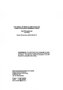
not be reachable in practice. We assume that the fraction of such enumerables is negligible. Figure 1 [31] shows the relationship among some well-known criteria as proven by Weyuker. If there is a directed path from criteria A to criteria B , then test sets that meet criteria A (achievement of complete coverage) are guaranteed to satisfy criteria B. Table 1 shows the maximum number of tests [31] to satisfy these criteria and the observed complexities [30] for some specific cases. The upper bound for all-du-paths was reached in one subroutine out of 143 considered by Bieman and Schultz [bisc89,bisc92]. AlCPsths
Table 1: The complexity (test length) for achieving different coverage criteria [31] Coveraee Criterion
IAll-Blocks
I U D D e r bound I Observed I id+ 1
All-Branches All-P- U ses
Id+l
I
I
1
I f(d2 + 4d + 3) I0.38d + 3.17
All-DU-Paths
2d
All-Paths
CO
2d
B All-DU-Paths
AII-U~S
AICC-Uses SombP-Uses
All-P-Uses SomeC-Uses
%&B
AICP-Uses
B B
All-Branches
AlCBlocks
Figure 1: The subsumption relationships of different complete coverage criteria [31] To keep the following discussion general, we will use the term enumerable. For branch coverage, the enumerables are branches, for defect coverage the enumerables are defects and so on. We use the term “enumerable-type” to imply defects, blocks, branches, c-uses or p-uses. We use superscript i , i = 0 to 4, to indicate one of the five types in this sequence: 0: defects, 1: blocks, 2:branches, 3: c-uses, 4: p-uses.
3
Detectability Profiles of Enumerables
The coverage achieved by a set of tests depends not only on the number of tests applied (or, equivalently, the testing time) but also on the distribution of testability values of the enumerables. A statement which is reached more easily is more testable. Such
statements are likely to get covered (i.e. exercised at lease once) with only a small number of tests. Testability also depends on the likelihood that a fault that is reached actually causes a failure [27]. A statement that is executed only in rare situations has low testability. It may not get exercised by most of the tests that are normally applied. As testing progresses, the distribution of testability values will shift. The easyto-test enumerables are covered early during testing, and are removed from consideration. The remaining enumerables include a larger fraction of hard-to-test enumerables. Thus, the growth of coverage will be slower. Definition: Detectability of an enumerable d{ is the probability that the I-th enumerable of type j will be exercised by a randomly chosen test. The detectability profile is the distribution of detectability values in the system under test. The detectability profiles were introduced by Malaiya and Yang [15]. They have been used to characterize testing of hardware [29] and software [19]. A continuous version of the detectability profile was defined by Seth, Agrawal and Farhat [25]. For convenience, we use the normalized detectability profile (NDP) as defined below. Definition: The discrete NDP for the system under test is given by the vector,
pi = {dl,d2, ...,di,...,d,’, where di is the fraction of all enumerables of type j which have detectability equal to di. Thus p i , 3 represents the fraction of all branches with detectability of 0.3. In Equation 1, du is the detectability value of unity ( l ) ,the highest value possible. = 1 since all fractions added will be unity. A detectability value of 0 is possible, since a branch might be infeasible, or a defect might not be testable
cii=op$i
with detectability d: will not be covered is ( 1 - d i ) . The probability that an enumerable will not be covered by n tests and thus remain a part of profile is ( 1 - d: )" . Thus if the initial profile was given by Equation l , the profile after having applied n tests, will be given by
due to redundancy in implementation. Researchers have compiled detectability profiles of several digital circuits [15, 291 and software systems [26, 71. If the number of enumerables is large, a continuous function can approximate the discrete NDP. Definition: The continuous NDP, for the system under test is the function p ' ( x ) , 0 5 x 5 1 pl(x)dx =
nr-enumerabled ( x , x all-enumerablesj
+dx)
(2)
Equivalently the continuous profile is given by
where n r _ e n u m e r a b l e d ( x ,x + d x ) denotes all enumerables of type j with detectability values between x and x dx. p J ( x ) d x = 1,just like the discrete NDP case.
A(.) = P n ( x ) ( l -
+ s,'
4
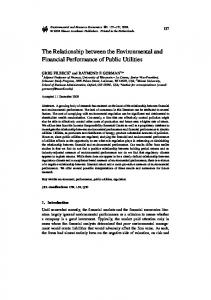
Thus enumerables with high testability are likely to get covered earlier. The profile will "erode" as testing progresses (see Figure 2). Enumerables with low testability get removed at a much lower rate, and thus will soon dominate. During much of the testing, the shape of the profile will appear like the bottom curve in Figure 2, regardless of the initial profile. Available results for hardware components suggest that initial detectability profiles may be of the form
A one-parameter Model
The detectability profile gives the probability of exercising each enumerable. Hence, it can be used to calculate expected coverage when a given number of tests have been applied. Here, we assume that testing is random, i.e. any single test is selected randomly with replacement. Malaiya and Yang [15],and Wagner et a1 [29] show that the expected coverage of the enumerables of type j is
(5)
+
where m j is a parameter. The factors ( m j 1 ) ensure that the area under the initial profile curve is unity. By substituting the right hand side of Equation 5 in Equation 4, we get
n
C j ( n )= 1 - c ( 1 - d { ) " d
(3)
i=l
C j ( n )= 1 - ( m j
provided testing is random. The same result holds for continuous NDP [25] C j ( n )= 1 -
l1(l
-XYP(X)dX
x)"
=I-
(4)
+ 1)
1'
mj+1 mj+n+l
( 1 - x)mj+ndx
-
n mj+n+l
(6)
The curve given by Equation 6 matches the shape of experimental data. However it does not provide a good fit. One problem is that Equation 6 includes only a single parameter which can be adjusted for fitting. We can assume a more general initial detectability in Equation 5 , involving two parameters, but even that may not be accurate, as we discuss in the next section. The approach considered next, yields a much better model.
Actual testing of software is more likely to be pseuderandom, since a test once applied will not be repeated. In such cases, random testing is an approximation. This approximation is reasonable, except when coverage approaches 100%. Equations 3 and 4 give expected coverage. In a specific case, the coverage can be different. The central limit theorem suggests that results obtained should be close to these given by Equations 3 and 4 when a large number of vectors are applied. The use of Equations 3 and 4 requires knowledge of detectability profiles. Obtaining exact detectability profiles requires a lot of computation. Discrete detectability profiles have been calculated for several small and large combinational circuits. Continuous detectability profiles for some benchmark circuits have been estimated [25]. However software systems are generally much more complex. Fortunately, it is possible to obtain reasonable approximation for the detectability profiles. When one test is applied, the probability that an enumerable
5
A New Logarithmic Coverage Model
Random testing implies that a new test is selected regardless of the tests that have been applied thus far, and that tests are selected based only on the operational distribution. In actual practice, a test case is selected in order to exercise a functionality or enumerable that has remained untested so far. This process makes actual testing more directed and hence more efficient than random testing.
189
2
at time m at time 11 at tlme 13
1.8
I....
-
1.6 1.4
'.
. . , ,
1.2 1
I %
% I
. -
-
:
\ \
.
,.
I
*\
.
I
. ..
I I>
',
. ..
,,
I
>\
,\
0.8 0.6 0.4
0.2 0
0.2
0
0.4
0.6
Detectability
0.8
Figure 2: Distribution of detectability and
Malaiya, von Mayrhauser and Srimani [18] show that this non-random process leads to a defect finding behavior described by the logarithmic growth model [17]. Their analysis gives an interpretation for the model parameters. The coverage growth of an enumerable-type depends on the detectability profile of the type and the test selection strategy. If the defect coverage growth in practice is described by the logarithmic model, it is likely that the coverage growth for other enumerable-types is also logarithmic. We suggest the following model. 1
~ ' ( t=) -,B; N'
'
ln(l+
pit),
cyt)5 1
p," = u0 (10) where K o ( 0 ) is the exposure ratio at time t = O , TL is the linear execution time and u0 is a parameter that describes the variation in the exposure ratio. Equation 8 relates coverage C' to the number of tests applied. We use it to obtain an expression giving defect coverage CO in terms of one of the coverage metrics C', i = 1 to 4. Using Equation 8, we solve for n, 1 C' - [ e z p ( - )bb n = b',
(7)
i = l to 4
- I],
Substituting for Colagain using Equation 8,
where Nf is the total number of enumerables of type i , Poand PIare model parameters. If a single application of a test takes T, seconds, then the time t , needed to apply n tests is nT,. Substituting in 7,
CO = bo0 ln[l
+ +bo( e z p (C'F ) b,
bo
- l)],
8
i = l to 4
k, we can
Defining ut = b!, U'; = and U $ = write the above using three parameters as, Defining bb as the above as,
(3) and b'; as (P;T,),we can rewrite
C'(n) = b6 ln(1
+ bfn),
C i ( n )5 1
i = 1 to 4 (11) Equation 11 gives a convenient three-parameter model for defect coverage in terms of a measurable test coverage metric. Equation 11 is applicable for only CO 5 1. It is possible to approximate Equation 11 using a linear relation, but it would be accurate for only a small range. CO
(8)
When C' = 1, there are no more additional enumerables of that type to be found. With non-random testing a finite, although possibly large, number of tests are required to achieve 100% coverage of the feasible enumerables. For defects (i = 0), the parameters and have the following interpretation [19].
6
= a6 l n [ l + a f ( e z p ( u $ C ' ) - 111
Analysis of Data
We evaluate the proposed model, as given by Equations 8 and 11, using four data sets. The first data
(9)
190
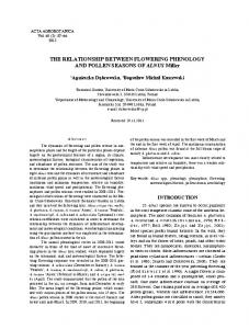
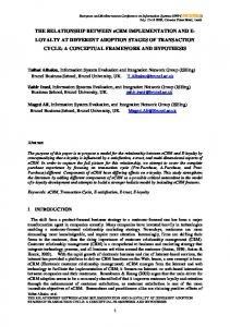
tent p-use coverage, are both strongly correlated with block coverage. The correlation with c-use coverage is weaker. Figure 4 shows actual and computed values for fault coverage. The computed values have been obtained using branch coverage and Equation 11. At 50% branch coverage the fault coverage is still quite low (about IO%), however with only 84% branch coverage, 90% fault coverage is obtained. The branch coverage shows saturation at about 84%. This supports the view that 80% branch coverage is often adequate [IO]. Figure 5 is a scatter plot of computed values of defect coverage against actual values. The computed values are from the number of tests and Equation 8 (traditional reliability growth modeling), and test coverage measures C', C2,C3 and C4using Equation 11. The calculated values are all quite close, showing that coverage based modeling can replace time-based modeling.
set, DS1, is from a multiple-version automatic airplane landing system [14]. It was collected using the ATAC tool developed at Bellcore. The twelve versions have a total of 30,694 lines. The data used is for integration and acceptance test phases, where 66 defects were found. One additional defect was found during operational testing. The second data set, DS2, is from a NASA supported project implementing sensor management in inertial navigation system [28]. For this program, 1196 test cases were applied and 9 defects were detected. The third data set, DS3, is for a simple program used to illustrate test coverage measures [l]. The fourth data set, DS4, is from an evolving software system containing a large number of modules. Table 2: Summary table for DS1 (total 21,000 tests applied)
I Blocks I Decisions I Find cov.
LSE
91.8% 0.031 2E+8 5.7E4
I
I
c-uses p u s e s Defects
I
Table 4: Summary table for DS3 (total 16 tests applied)
83.9% 91.7% 73.5% 98.4% 0.049 0.036 0.041 0.184 1234 3.4E+6 2439 0.01 3.53-5 5.83-4 8 . 1 6 5 7 . 3 E 7
i= 1
Table 3: Summary table for DS2 (total 1196 tests applied)
I
I bf
LSE
I
0.061 8.435 2E-5
I
I
0.111 0.111 0.121 769 561 162 1.7E-3 1 . 6 E 3 2.33-3
Table 4 shows similar results for a very small illustrative program. No defects were involved. However, this again demonstrates the applicability of our modeling scheme. We see that C1 2 C2 C4. The c-use coverage again behaves differently. In evolving programs, significant changes are being made while testing is in progress. Because new modules are being added, new defects as well as noncovered enumerables are also being added. The coverage obtained by a test set can actually go down in some cased. From DS4, (see Figure 6 ) , the linear correlation between coverage measures can still be applicable. The data used here covers an intermediate phase of the process. The analysis of evolving programs is more complex and is the subject of future research.
6.95
>
The first data set and the results from it are summarized in Table 2. The first row gives the total number of enumerables for all versions. The second row gives the average coverage when 21,000 tests had been applied. The values of the estimated parameters 6; and bi and the least square error are given in the rows below. The model given by Equation 8 fits the data well. The data shows that C' > C2 > C4. This relationship is expected. Complete decision coverage implies complete block coverage, and complete p-uses coverage implies complete decision coverage [2, 8, 201. The c-uses coverage has no such relation relative to the other metrics. Indeed the data shows that while C3 < C' at the beginning of testing, near the end of testing C3 is almost equal to c1. Table 3 summarizes the result for DS2. Nine faults were revealed by application of 1196 tests; we assume that one fault (i.e. 10%) is still undetected. In spite of the small number of faults, the model given in Equations 11 fits the data well.
7
Model Parameters
Researchers find that the logarithmic model works best among other two-parameter models [16], however interpretation of its parameters is difficult. One interpretation given by Malaiya et a1 [18] is described by Equations 9 and 10. The same interpretation may be applicable for enumerables other than defects. The first parameter of Equation 8 is,
Figure 3 shows the correlation of other test coverage measures Cz, C3 and C4 with block coverage C' . As we expect, branch coverage, and to a lesser ex-
191
0.9
0.6
0.55
0.7 0.75 Block Coverage
0.65
0.8
0.9
0.85
Figure 3: Scatter plot of C2, C3 and C4 against C1 0.9 0.8 0.7
0.8
0.5
0.4
0.3 0.2 0.1
I 0.5
0.45
0.55
0.8
0.65
Branch Coverage
0.7
0.75
0.85
0.8
Figure 4: Actual and fitted (using Equation 11) values of defect coverage .
K'(0)N' - K ' ( 0 ) =aaTrNi a'Tr & .
Y
and a i is as an initial estimate for numerically fitting Equation 11, the initial estimate itself provides a least-square fit. If the initial estimates are significantly different, then the least square fit may iield somewhat different parameter A-priori estimation of model parameters remains a partly unsolved problem. Currently we must rely on curve fitting based approaches.
(12)
The linear execution time is given by the number of lines of code multiplied by the average execution time Of each line. An empirical method to estimate the initial fault exposure ratio K o ( 0 ) has been suggested by Li and Malaiya 1121. Estimation of a' remains an open problem. The second parameter is given by,
6' = aoT,
8
(13)
The single test execution time T, depends on the program size and its structure. The product bgbi then should be independent of the program size. The parameters U;, a i , and a i are defined in terms . . of bb and bf above. When this definition for ab, a;,
Defect density and reliability
Since the failure intensity is proportional to the number of defects, we have [1g, 191,
Ii'
A=-N TL
192
1
0.8
-
n-fi c bk-fi -t-. br-fi - e - =-fi ..y..... p-fi 4.y=x -
. ...........*LZL
0.6
0.4
0.2
0 0
0.2
0.6 Actual Fault Coverage
0.4
0.8
Figure 5: Actual defect coverage vs computed values 44
real data e fitted line -
Figure 6: Scatter chart for module & branch coverages for an evolving program Equation 14 can also be used for operational period using the appropriate value for the fault exposure ratio. Notice that K will depend on the operational profile used.
Where K is the overall value of fault exposure ratio. Let NO be the total number of faults initially present in the program and there is no new fault introduced during testing process. Then N can be computed as:
9
N = No(1 -CO)
We developed a modeling scheme that relates defect density to measurable coverage metrics. Defects have a detectability distribution like other coverage enumerables, and the same model may govern them. TWOadvantages of using a logarithmic model to describe test effort and enumerables covered are:
Substituting CO using Equation 11,
N = NO(I - ut I n [ l + uf(ezp(uiC1) - 111) Hence, the expected duration between successive failures can be obtained as 1 1 - TL A K NO(1 - u t h [ l +u i ( e z p ( u i C i )- I)])
Conclusions and Discussions
1. The logarithmic model is superior to other models for predicting the number of defects.
(14)
193
Our results can serve as a basis for further data collection and analysis. We need to examine the behavior a t different fault densities, especially at very low defect densities (for highly reliable applications). We also need to validate the model for different, testing strategies on the modeling scheme and the parameter values. In general, deterministic (coverage driven) is more efficient than true random testing. Testing using special values or use of equivalence partitioning can significantly compress the test time. Since test coverage measures provide direct sampling of the state of the software, we expect Equation 11 to hold because time is eliminated as a variable. Additional data will allow us to validate and refine our modelling scheme. In addition we need to develop schemes for evolving programs where new faults and other non-covered enumerables are being added.
2. The logarithmic model can account for 100% coverage achieved in finite time. For high reliability applications, 100% block coverage night not be sufficient. A more strict coverage measure such as branch or p-use coverage can be used to further estimate the defect density. The data sets used suggest that the model works well. The results are consistent with the analytical coverage inclusion relationships. Our model is simple and easily explained, and is thus suitable for industrial use. The model given by Equation 11 can be used in two different ways. Extrapolation requires collecting data for part of the testing process, which is then used to estimate the applicable parameter values. These are used for making projections for planning the rest of the test effort. A priori parameter estimation requires empirical estimation of parameters even before testing begins. We have some observations on what factors control the parameter values. Further work is needed to fully develop these techniques and would include a careful study of enumerable exposure ratios. As we show, any test coverage measure can be used to estimate the defect density, by using applicable parameter values. This raises an important question. Should several coverage measures be used or just one? Which individual measure (or selected set) provides the best estimate?
10
Acknowledgement
We would like to thank Albert0 Pasquini, Bob Horgan, Aditya Mathur and Peng Lu for discussions on this subject.
References
We need further studies to determine which coverage measure provide the best estimates of the number of defects. For DS2, we find that block coverage C’ provides the best and c-uses coverage C3 the worst fit. This result may be true for only specific data sets, or for specific coverage/defect density ranges. Since the different coverage measures can be strongly correlated, perhaps they may work equally well in many situations.
H. Agrawal, J . Horgan, E. Krauser, S. London, “A testing-Based model and Risk Browser for C” Proc. Int. Conf. Rel., Q u d C o n t r o l l3 Risk Asses., Oct. 1993, pp 1-7. B. Beizer, Software Testing Techniques, Van Nostrand Reinhold, 1990, pp. 74-75, 161-171. J . Bieman and J . Schultz, “Estimating the Number of Test Cases Required to Satisfy the Alldu-paths Testing Criterion,’’ Proc. ACM TAV.9S I G S O F T , pp. 179- 186.
For very high reliability, we may need a “scale” that works in that region. If the requirements are such that 100% block coverage is not enough, branch or p-use coverage may be more appropriate. Branch coverage may be an adequate measure in many cases, since about 80% branch coverage often produces acceptable results [IO]. However for testing of individual modules or for highly reliable software p-use may be better.
J . Bieman and J . Schultz, “An Empirical Evaluation (and Specification) of the All-du-paths Testing Criterion,” Software Eng. J., Jan. 1992, pp. 43-5 1. M. Chen, J . Horgan, A. Mathur and V. Rego, “A time/structure based model for estimating software reliability,” SERC- T R - l l r - P , Purdue University, Dec. 1992.
Researchers suggests the use of a weighted risk measure [l, 23, 211. Weights are chosen on the basis of relative significance of each measure. As we find, structural coverage measures tend to be strongly correlated, and thus a weighted average may not provide more information than a single measure. We need to identify more independent measures. Other types of coverage measures like functional coverage may be suitable.
S. Dalal, J . Horgan and J . Kettenring, “Reliable Software and Communications: Software Quality, Reliability and Safety,” Proc. 15th Int. Conf. Software Eng., May 1993, pp. 425-435
194
J . Dunham, “Experiments in software reliability: Life Critical Applications,” IEEE Trans. Soft. Eng., Jan. 1986, pp. 110-123.
[20] S. Ntafos, “A Comparision of Some Structural Testing Strategies” IEEE Trans. Software Eng., June 1988, pp.868-874.
P. Frankl and E. Wayuker, “An Applicable Family of Data Flow Testing Criteria,” IEEE Trans. Soft. Eng., Oct. 1988, pp. 1483-1498.
(211 A. Neufelder, Ensuring Software Reliability, Marcel Dekker Inc., 1993, pp. 137-140. [22] P. Piwowarski, M. Ohba and J . Caruso, “COVerage measurement experience during function test ,” ICSE’99, pp. 287-300
P. Frankl and N . Weiss, “An Experimental Comparison of the Effectiveness of Branch Testing and Data Flow Testing,’’ IEEE Trans. Soft. Eng., Aug. 1993, pp. 774-787.
[23] R. Poston, “The Power of Simple Software Testing Metrics”, Software Testing Times, Vol. 3, No. 1993.
R. Grady, Practical Software Metrics for Project Management and Process improvement, P T R Prentice-Hall, 1992, pp. 58-60.
[24] J . Ramsey and V. Basili, “Analyzing the Test Process Using Structural Coverage”, Proc. ICSE’85, pp, 306-312.
H. Hecht and P. Crane, “Rare Conditions and Their Effect on Software Failures,” Proceedings of Ann. Reliability and Maintainability Symp., pp. 334-337, Jan. 1994.
[25] S. Seth, V. Agrawal and H. Farhat, “A Statistical Theory of Digital Circuit Testability,” IEEE Trans. Comp., Apr. 1990, pp. 582-586.
N. Li and Y. Malaiya, “Fault Exposure Ratio and Reliability Estimation,” Proc. 3rd Workshop Issues Software Reliability, Nov. 1993, pp. 6.3.16.3.18.
[26] M. Trachtenberg, “Why Failure Rates observe Zipf’s Law in Operational Software,” IEEE Trans. Reliability, Sept. 1992, pp. 386-389. [27] J . Voas and K. Miller, “Improving the Software Development Process Using Testability Research,” ISSRE’92, pp. 1 14- 12 1.
N. Li and Y. Malaiya, “Enhancing Acuracy of Software reliability Prediction” ISSRE’93, pp. 7179. M. Lyu, J . Horgan and S. London, “A Coverage Analysis Tool for the Effectiveness of Software Testing” ISSRE’93, pp. 25-34.
[28] M. Vouk “Using Reliability Models During Testing With Non-operational Profiles,” Proc. 2nd Bellcore/Purdue workshop issues in Software Reliability Estimation, Oct. 1992, pp. 103-111
Y. Malaiya and S. Yang, “The Coverage Problem for Random Testing,” Proc. Int. Test Conference, pp. 237-242, Oct. 1984.
[29] K. Wagnor, C . Chin and E. McCluskey, “Pseudorandom Testing,” IEEE Trans. Comp., Mar. 1987, pp. 332-343. [30] E. Weyuker, “An Empirical Study of the Complexity of Data Flow Testing,” Proc. TAV2, July 1988.
Y. Malaiya, N. Karunanithi and P. Verma, “Predictability of Software Reliability Models,” IEEE Trans. Reliability, Dec. 1992, pp. 539-546.
[31] E. Weyuker, “More Experience with Data Flow Testing”, IEEE Trans. Soft. Eng., Sept. 1993, pp. 9 12-9 19.
[17] J. Musa, A. Iannino, K . Okumoto, Software Reliability, Measurement, Prediction, Application, McGraw-Hill, 1987. [18] Y. Malaiya, A. von Mayrhauser and P. Srimani, “The Nature of Fault Exposure Ratio,” Proc. IEEE Int. Symp. Soft. Rei. Eng., Oct. 1992, pp. 23-32. [19] Y. Malaiya, A. von Mayrhauser and P. Srimani, “An Examination of Fault Exposure Ratio,” IEEE Trans. Software Eng. Nov., 1993, pp. 1087-1094.
195