the robustness of pi & pid controllers in the presence of sampling jitter

THE ROBUSTNESS OF PI & PID CONTROLLERS IN THE PRESENCE OF SAMPLING JITTER Wei Yu, ∗ David I. Wilson, ∗∗ Jonathan Currie, ∗∗ and Brent R. Young ∗∗∗ ∗

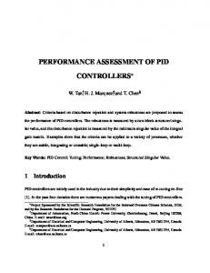
Industrial Information & Control Centre, The University of Auckland, New Zealand ∗∗ Electrical & Electronic Engineering, Auckland University of Technology, New Zealand ∗∗∗ Chemical & Materials Engineering, The University of Auckland, New Zealand Abstract: Variations in sampling time, or sampling jitter, is a common industrial control problem. This paper investigates the performance of industrial PI and PID controllers in the presence of sampling jitter. The commonly employed controller performance assessment (CPA) benchmark index is used on a wide variety of industrial plant models to show that while the PI control is relatively immune to jitter, the derivative component of the PID controller causes the PID controller to exhibit excessive sensitivity to sampling jitter, although this can be partially compensated by appropriate filtering. Keywords: Robustness of PID controllers, Sampling jitter, Performance index 1

Introduction

Many real-time control systems are implemented as distributed control systems where the digital feedback control of continuous plants is over a communication network or a field bus. While the controller supposedly works at a fixed nominal period, varying computer load, unexpected delays and other unforseen issues all contribute to a system that experiences a stochastic sampling rate known as sampling jitter. This paper investigates the relative deterioration in the quality of control for common controllers operating in this situation. Jitter problems have been traditionally identified as important in high-speed communication and signal processing applications. Jitter detection and measurement were addressed in Liu [1991] and Sharfer and Messer [1994]. Jitter modeling and identification have been studied in Ou et al. [2004],Boje [2005],Eng and Gustafsson [2008] and Burnham et al. [2009] and the controlling of systems with jitter problems can be found in Sala [2005] and Nilsson et al. [1997]. Specific applications such as controller jitter compensation were discussed in Lincoln [2002] and Niculae et al. [2008]. PID controllers are the most commonly employed industrial feedback controller due to their simplicity of implementation, and (despite the continuing plethora of research activity), relative ease of tuning. In this paper, we will investigate the control performance of the PI and PID controllers given sampling jitter. Control performance assessment, or CPA, is a technology employed to diagnose and maintain operational efficiency of control systems developed in a direct response to address this increasingly important economic problem. Linear CPA is routinely applied in the refining, petrochem⋆ To whom all correspondence should be addressed.

icals, pulp and paper and the mineral processing industries as noted by T.J. Harris [1999] and Huang and Shah [1999], while practical overviews are given in Qin [1998], M. Jelali [2006] and Hoo et al. [2003] and an automated system intended for plant wide use is described in Scali et al. [2009]. In this paper, one control benchmark, the minimum variance lower performance bound, is used to quantify the PI and PID controller performance. Linear systems corrupted with sampling jitter can be expressed as linear time-varying systems. CPA has previously been addressed to the time-varying systems in which the time-varying coefficients were expressed as time functions in Huang [2002] and Olaleye et al. [2004]. We should mention that the time varying systems studied in this paper are different to these systems as the coefficients of the time varying systems are stochastic variables caused by the random sampling period. A related problem common in control systems with wireless links is analysed in Song et al. [2006] where they propose modifying the derivative component of the PID controller to avoid excessive derivative kick and integral windup when the wireless link has failed. The layout of the paper is as follows. Section 2 introduces the system under consideration in this paper and section 3 justifies the choice of using the minimum variance lower bound as a performance index. Section 4, compares, using a collection of representative plant models, the robustness of PI and PID controllers given differing sampling jitter. Finally, section 5 concludes with general statements about controllers and jitter and some future directions. 2

Process Formulation

In the following development we must make some assumptions regarding the shape of the probability distribution (PDF) of the sampling jitter. An obvious jitter

PDF is uniform or Gaussian about some nominal sample rate. However in many cases it may be more realistic to have a PDF distribution with a significant tail towards the longer periods such as exponential. The motivation for these types of distributions is due to the fact that at the times when significant control calculations are needed is when good control is also needed. Some controllers with a constant structure and operation count (such as PID) are independent of state (except when transferring from auto to manual), while others such as MPC take longer to solve the embedded optimisation problem when recovering from upsets, or moving to a new setpoint. The embedded MPC controller in Currie and Wilson [2010] illustrates this by taking 5 times as long when solving the constrained optimisation problem compared to when the unconstrained controller is active. Finally in many instances a single chip will be controlling a number of loops, so a time out in any one loop will cause interrupts to be missed in the others. We will assume a PDF for the jitter, where the sampled signal, yk , are taken at time instances tk = tk−1 +(T +τk ), where T is the nominal constant sampling interval, and the jitter component, τk > 0, is a family of identically distributed independent random variables. In this paper we will consider two specific distributions for the sample jitter; a uniform distribution with τ ∈ U(0, τmax ), and an exponential distribution which is theoretically unbounded on the right. For the purposes of the simulation study in this paper, we assume that the output of the process is sampled with a stochastic sample time, that the control signal is applied to the process as soon as the data arrives, and that the actual sampling period is always greater than, or equal to, the nominal sample time, T . The last assumption, a consequence that we have only considered the cases where τk > 0, is simply from the practical consideration that for industrial control systems are never early since they will wait until the appropriate interrupt, but can get delayed. The timing of signals in the control system with the sampling jitter problem is illustrated in Fig. 1 where the first diagram shows the process output and the samples with a constant sampling period T , the second diagram illustrates the exact signal recorded with the jitter sampling situation, and the third diagram shows the process inputs.

6 y

6 yk 6 uk (k − 1)T

kT

(k + 1)T

Figure 1. Signals of a control system with the sampling jitter problem

Given a single-input single-output (SISO) continuous time (CT) system y(t) = G(s)u(t) (1) where for simplicity G(s) has n distinct poles, n ∑ ci G(s) = e−f s (2) s − λ i i=1 where we sample at instants tk ∈ R, k = 0, 1, · · · , with tk+1 > tk , t0 = 0. The time-varying sampling period will be denoted by Tk = T + τk , and it will be assumed to lie in a known compact set J. Given the output at time tk , y(tk ), if the input u(tk ) is kept constant across the inter-sampling interval, the output at time tk+1 is, y(tk+1 ) = G(q −1 )q −f +1 u(tk ) (3) −1 −1 where q is the backshift operator, q yk+1 = yk . The discrete transfer function is n ∑ 1 eλi Tk GTk (q −1 ) = ci · (4) λi Tk q −1 λ 1 − e i i=1 Introducing the notation Gk (q −1 ) = GTk (q −1 ), y(tk+1 ) = yk+1 and u(tk ) = uk , the system in Eq. (3) can be succinctly expressed as, yk+1 = Gk (q −1 )q −f +1 uk Bk (q −1 ) −f +1 = (5) q uk Ak (q −1 ) where Ak (q −1 ) and Bk (q −1 ) are time-varying polynomials (due to the time-varying sampling rate), and f is the time delay of the system which is assumed known. If there is an additive disturbance dk , the total process can be written as, Bk (q −1 ) −f yk = q uk + dk (6) Ak (q −1 ) where dk can be modelled as the output of a linear Autoregressive-Integrated-Moving-Average (ARIMA) filter driven by white noise ak of zero mean and variance σa2 of the form θ(q −1 ) dk = ak (7) ϕ(q −1 )∇h where ∇ = (1 − q −1 ) is the difference operator and h is a non-negative integer, typically less than 2. The polynomials θ(q −1 ) and ϕ(q −1 ) are monic and stable. The control performance assessment for the more general LTV SISO in which the disturbance is also time varying can be found in Huang [2002]. In this paper, we will assume that the disturbance distribution is time invariant. 2.1 Control realisation Commercial PID controllers filter the derivative component to avoid amplifying high frequency noise. One common realisation is ) ( τd s 1 + sτd (8) C(s) = K 1 + τi s N +1 where the derivative filter time constant N is factory set in the region of 2 to 100, [˚ Astr¨om and H¨agglund, 2006, p73]. Since sampling jitter is going to adversely effect the derivative-type terms in a controller, the precise discrete realisation, and value of N are crucial. In this paper, we discretise the controller in Eqn. 8 with a zeroth-order hold and compare the case with N → ∞ (a pure PID controller) with the industrially typical N = 10.

Pf (q −1 ) is a polynomial obtained by solving the Diophantine equation: −1 θ(q −1 ) ) −1 −f +1 −f Pf (q = 1+φ q +· · ·+φ q +q 1 f −1 ϕ(q −1 )∇h ϕ(q −1 )∇h (13) When employing minimum variance control, the first two terms in Eq. (9) equal zero, so the now minimum variance output is simply MV = ek+f |k (14) yk+f The MVPLB in the mean square sense can expressed as, 2 MV σMV = var{yk+f } = (1 + ψ12 + · · · + ψf2 −1 ) σa2 (15) and a performance index defined as σ2 η = MV (16) σy2 can be used to quantitatively rank the controlled performance of the PI/PID controllers. Since the system in Eq. (6) is a time varying system, it will be very difficult to estimate η reliably directly from the output data. In this paper however, we will not address 2 this problem, so we will assume we know σMV . While this assumption may appear unrealistic, the purpose of this paper is simply to compare the controlled performance of these stochastically time-varying systems under different control strategies.

4

Simulation experiments

In this section, we test the robustness of PI and PID controllers disturbed by differing amounts and types of jitter when applied to a collection of 12 typical representative

1 PI control

0.5 yk (PI)

−1

θ(q ) the φ weights are the impulse coefficients of the ϕ(q −1 )∇h transfer function, and Bk+f (q −1 ) Pf (q −1 ) yk+f |k = u + ak k Ak+f (q −1 ) ϕ(q −1 )∇h Bk+f (q −1 ) Pf (q −1 ) = u + (yk − yˆk|k−1 ) k Ak+f (q −1 ) ϕ(q −1 )∇h (12)

0 −0.5 −1 1 PID control

yk (PID)

To quantitatively assess the performance of various controllers under typical industrial conditions we propose using the minimum variance performance lower bound (MVPLB) originally proposed by T.J. Harris [1989]. This index is the ratio of the best achievable variance of any controller to the actual measured variance of the controlled variable under assessment. However, standard CPA analysis assumes regular sampling, but this is not the case with jitter. To obtain the minimum variance performance lower bound (MVPLB) for the system in Eq. (6), we only need to show that the f -step ahead prediction error, ek+f |f , is independent of the manipulated variable action. The feedback invariant is given in Bk+f (q −1 ) uk + dk+f |k + ek+f |k (9) yk+f = Ak+f (q −1 ) = yk+f |k + ek+f |k (10) where ek+f |k = (1 + φ1 q −1 + · · · + φf −1 q −(f −1) ) ak+f , (11)

industrial plant models collected from H¨agglund [2002] and Skogestad [2003], but where we added additional time delay as listed in Table 1. The parameters of the PI and PID controllers are calculated using the SIMC-PID tuning method from Skogestad [2003], and adjusted to PID controllers in the ISA or parallel form. We consider two types of disturbance signals; one lowpass and one high-pass filtered white noise sequence  ak  low-pass −1 1 − 0.8q dk = (17) a k  high-pass 1 + 0.8q −1 where ak is a sequence of i.i.d. Gaussian random variable with zero mean and constant variance σa2 = 0.01. The simulation outputs of the process model P 1 with disturbance model 1 corrupted with the sampling period distributed uniformly in the range from T to 3T , (or Tk ∈ U[0.05, 0.075]) is shown in the left-hand column and the case with exponentially distributed jitter in the right hand plot of Fig. 2. The top trend shows the PI controlled output, while the middle trend shows the PID controlled output, both using the tuning values listed in Table 1. The lower two trends shows the actual varying sample time, and its distribution.

0.5 0 −0.5 −1

k

A performance index for jitter cases

Sample time: T

3

0.1

0.05

0

0

0.05

50 100 150 Sample time, k

0.06 0.07 Sample time

200

0.08

0

0.06

50 100 150 Sample interval, k

200

0.08 0.1 0.12 Sample time

0.14

Figure 2. The PI and PID controlled outputs and jitter sampling plots for system P1 for both a uniform (left column) and an exponential (right column) distribution of sampling jitter. The results presented in Fig. 2 are for a specific model and a specific nominal range of uniform jitter. Generalising on these results, Fig. 3 shows for all 12 plants listed in Table 1, the performance index, η, from Eqn. 16 as a function of increasing uniformally distributed jitter from no jitter, τmax = 0, to substantial jitter, τmax = 2 corresponding to a range of sample times spanning from

Table 1. A collection of 12 industrial process models with sampling time, T , and appropriate PI and PID tuning constants. Case

P1

Process model

T

e−0.1s (s + 1)(0.2s + 1)

0.05

P2

(−0.3s + 1)(0.08s + 1)e−0.3s (2s + 1)(s + 1)(0.4s + 1)(0.2s + 1)(0.05s + 1)3

P3

2(15s + 1)e−0.2s (20s + 1)(s + 1)(0.1s + 1)2

P4

e−1.5s (s + 1)4

0.1

0.5

P5

e−0.4s (s + 1)(0.2s + 1)(0.04s + 1)(0.008s + 1)

P6

(0.17s + 1)2 e−0.2s s(s + 1)2 (0.028s + 1)

P7

(−2s + 1) e−0.45s (s + 1)3

P8

e−0.3s s(s + 1)2

P9

e−2.5s (s + 1)2

P10

e−2.5s (20s + 1)(2s + 1)

P11

(−s + 1)e−2s (6s + 1)(2s + 1)

P12

(2s + 1)e−1.3s (10s + 1)(0.5s + 1)

T to 3T . Fig. 4 shows the average performance across all models for the low-pass and high-pass filtered noise cases. The trends for the cases with exponentially distributed jitter are similar. From these results, (and equivalent tests using exponentially distributed jitter noise and bimodal distributed jitter noise not shown in this paper), we can observe that: • For the majority of the plants considered, the controlled performance of PID is superior to PI if there is no sampling jitter (which is as expected). • For PI control, the controlled performance deteriorates relatively slowly with increasing sampling jitter. This indicates that PI controllers are relatively immune to fluctuations in sampling time. • On the other hand, the the controlled performance for PID control deteriorates significantly more rapidly with increasing sampling jitter. Consequently this suggests that PID control is not a good choice when the control loop experiences sampling jitter. • Controllers which filter the derivative component partially compensate the problems with sample jitter.

0.1

0.02

0.1

0.15

0.1

0.5

0.5

0.25

0.15

Kc

Controller τI

2.75

1.1

–

6

1.2

0.167

0.706

2.5

–

1.984

2.27

0.566

1

1.05

–

1.53

1.15

0.13

0.188

1.5

–

0.417

2.5

0.6

2.93

1.1

–

10.46

0.74

0.155

0.265

15.12

–

1.16

5.79

1.02

0.19

1.5

–

0.4223

1.5

1

0.278

14.4

–

0.937

9.6

2.13

τD

0.25

1.5

–

0.666

2

0.5

3.5

21

–

4.4

22

1.82

0.583

7

–

1.12

9

2

2.32

4.5

0

3.15

6.1

0.1

It is not unexpected that control algorithms that involve finite differencing of measured signals are particularly suspect to jitter. Clearly if the control algorithm has significant gain at the higher frequencies, and the disturbances exhibit significant high-frequency component such as in the case with a high-pass filtered noise, then slight errors in timing (which is essentially the same as high frequency disturbances) will have a disproportionate effect. This explains why the (unfiltered) derivative component of the PID controller causes the rapid deterioration in performance where for some plants η → 0, indicating that the output variance σy2 → ∞. The problem is particularly insidious when trying to control those processes that need some derivative action to stabilise such as double integrators. This could also be an issue for those automated PID tuning algorithms that also adjust the ‘factory-set’ filter time constant N in Eqn. 8. It was mentioned in section 1 that jitter has been traditionally of concern only in high-speed computer networks rather than low speed process control applications. However there are a number of current trends in the processing

Uniformally distributed jitter: Low−pass filter

P1

P2

P3

P4

P5

P6

P7

P8

P9

P10

P11

P12

PI PID PID

N=10

0.5

1

1.5

2 0

0.5

1

1.5

2 0

0.5

1

1.5

2 0

0.5

1

1.5

2

Upper bound of sampling period [τmax]

Figure 3. The degradation of the control performance, η, for the 12 plants under consideration using PI (—⋄—) and PID, (—◦—), and PID with D-filter, N = 10, (· · · 2 · · · ) as a function of increasing sampling jitter magnitude. High pass noise filter

Low−pass noise filter 1 0.9 Average performance index, η

ak (1−0.8q −1 )

PI PID PID filterN=10

ak (1+0.8q −1 )

0.8 0.7 0.6 0.5 0.4 0.3 0.2 0.1

0.5 1 1.5 Upper bound of sampling period, [τmax]

2

0

0

0.5 1 1.5 Upper bound of sampling period, [τmax]

2

Figure 4. The average degradation of the control performance across all 12 candidate plants under consideration using PI (–⋄–) PID, (—◦—) and PID with a D-filter (2) as a function of increasing sampling jitter for low-pass filtered noise (left) and high-pass filtered noise (right). industries such as the fact that the time scales of interest are dropping, the increased use of high-order controllers such as LQR or MPC, and most importantly, the increased use of sophisticated process in-line, or at-line transducers that deliver rich measurements, but with imprecise time stamps. This too can be considered sampling jitter. Hence it is interesting to consider the robustness of the controller to this increasingly important problem. 5

Conclusion

The contribution of this work is to investigate the control performance degradation for systems with sampling jitter. We use a controller performance assessment index to quantify the degradation as a function of jitter magnitude, and we also investigated different plausible probability distributions for the jitter.

Clearly all controllers will be adversely effected by jitter, but those controllers that employ terms involving unfilterd finite differences in time such as the derivative control in PID controllers, and high-order controllers involving numerator dynamics are likely to be particularly vulnerable to this sort of disturbance. Acknowledgments Financial support for this project from the Industrial Information and Control Centre, Faculty of Engineering, The University of Auckland, New Zealand is gratefully acknowledged. References Karl J. ˚ Astr¨om and Tore H¨agglund. Advanced PID Control. ISA, Research Triangle Park, NC, USA, 2006.

E. Boje. Approximate models for continuous-time linear systems with sampling jitter. Automatica, 41:2091–2098, 2005. J.R. Burnham, C.K.K. Yang, and H. Hindi. A stochastic jitter model for analyzing digital timing – recovery circuits. In Proceedings of the Design Automation Conference 2009, pages 116–121, San Fraciscon, USA, July 2009. J. Currie and D.I. Wilson. Lightweight model predictive cotnrol intended for embedded applications. In Proceedings of the 9th International Symposium on Dyanimcs and Control of Process Systems, Leuven, Belgium, July 5–7 2010. Frida Eng and Fredrik Gustafsson. Identification with stochastic sampling time jitter. Automatica, pages 637– 646, 2008. K.J. H¨agglund, ˚ Astr¨ om. Revisiting the Ziegler-Nichols tuning rules for PI control. Asian Journal of Control, 4 (4):360–380, 2002. K. A. Hoo, M. J. Piovoso, P. D. Schnelle, and D. A. Rowan. Process and controller performance monitoring: overview with industrial applications. International Journal of Adaptive Control and Signal Processing, 17: 635–662, 2003. B. Huang. Minimum variance control and performance assessment of time-variant processes. Journal of Process Control, 12:707–719, 2002. B. Huang and S.L. Shah. Performance Assessment of Control Loops: Theory and Applications. Springer, 1999. B. Lincoln. Jitter compensation in digital control sytems. In Proceedings of the American Control Conference, pages 2985–2990, Anchorage, AK, May 2002. M.M.K. Liu. Jitter model and signal processing techniques for pulse width modulation optical recordingidentification with stochastic sampling time jitter. In Proceedings of the Communication, 1991, ICC91’, pages 810–814, Denver, USA, June 1991. M. Jelali. An overview of control performance assessment technology and industrial applications. Control Engineering Practice, 14(5):441–466, 2006. D. Niculae, C. Plaisanu, and D. Bistriceanu. Sampling jitter compensation for numeric PID controllers. In Proceedings of the Automation, Quality and Testing,

Robatics, 2008, IEEE International Conference, pages 100–104, May 2008. J. Nilsson, B. Bernhardsson, and B. Wittenmark. Stochastic analysis and control of real-time systems with random time delays. Automatica, 34:57–64, 1997. F.B. Olaleye, B. Huang, and E. Tarnayo. Feedforward and feedback controller performance assessment of linear time-variant processes. Journal of Process Control, 43 (2):589–596, 2004. N. Ou, T. Farahmand, A. Kuo, S. Tabatabaei, and A. Ivanov. Jitter models for the design and test of Gbps-speed serial interconnects. IEEE Design & Test of Computers, 21(4):302–313, 2004. S. J. Qin. Control performance monitoring - a review and assessment. Computer & Chemical Engineering, 23:173– 186, 1998. A. Sala. Computer control under time-varying sampling period: An LMI gridding approach. Automatica, 41: 2077–2082, 2005. Claudio Scali, Marco Farnesi, Raffaello Loffredo, and Damiano Bombardieri. Implementation and Validation of a Closed Loop Performance Monitoring System. In International Symposium on Advanced Control of Chemical Processes ADCHEM 2009, pages 78–87, Istanbul, Turkey, 12–15 July 2009. International Federation of Automatic Control. I. Sharfer and H. Messer. Feasibility study of parameter estiamation of random sampling jitter using the bispectrum. Circuits Systems Signal Process, 13:435–453, 1994. S. Skogestad. Simple analytic rules for model reduction and pid controller tuning. Journal of Process Control, 13:291–309, 2003. Jianping Song, Aloysius K. Mok, Deji Chen, Mark Nixon, Terry Blevins, and Willy Wojsznis. Improving PID control with unreliable communications. In ISA EXPO 2006, Houston, Texas, USA, 17–19 October 2006. ISA. T.J. Harris. Assessment of control loop performance. Canadian Journal of Chemical Engineering, 67:856–861, 1989. T.J. Harris. A review of performance monitoring and assessment techniques for univariate and multivariate control systems. J. Process Control, 9(1):1–17, 1999.