that the forces acting during the collision align the three atoms. The reaction probability at a .... theory based on statistical rather than dynamical assumptions is ...
Chemical
Physics 61 (19Sl)
North-Holland
189-204
Publishing Company
THE ROTATING ROD MODEL: OPACETY, EXCITATION, DEFLECTION FUNC’FIONS
FROM
COLLINEAR
AND ANGULAR
REACTION
DISTREBUTION PRO&ABILH?TIES*
Noam AGMON**‘f Department of Chemistry, Harvard Uniuersity, 12 Oxford Street, Cambridge, MA Received
02138,
USA
13 April 1981
A “rotating md” model for predominantly collinear atom-diatom collisions is presented. In this model it is assumed that the forces acting during the collision align the three atoms. The reaction probability at a given impact parameter is related to the 1D reaction probability by subtracting the triatomic rotational and bending energies from the total energy. An additional “sudden” approximation is used to derive a relation of deflection angles to impact parameters, resulting in an expression for angular distributions. Com@ison is made with quantal and classical trajectory calculations for HtHz and D-f-Hz and with trajectory calculations for Cl+ HD. A previously proposed analytical expression for ihe number of states along the reaction coordinate which gives a reasonable apprcximation for the collinear microcanonical reaction probability; is used for comparison with experiment. In this approximation all reaction attributes follow from the
diatomic spectroscopic constants and the “intrinsic barrier”, which is common to the reaction series. Comparison is made with angular distributions and excitation funcdon for D +H,. A simple, anaIytic expression derived for thermal rate constants Cl + HD.
is compared
with experimental
Arrhenius
plots for DiHz
1. Introduction A central goal of chemical
reaction
dynattics
reactions under single collision conditions. No experimental method approaches such conditions better than the (crossed) molecular beams technique [l. 21. This is the only method which enables one to measure the differential cross section, 1, as a function of the center of mass deflection angle, 8. It is frequently stated [3] that a backward peaked (19 = 180’) angular distribution for an exchange reaction A+ BC + AB + C is indicative of a direct reaction with preferred collinear configuration. The purpose of the present work is to examine this idea more quantitatively, by a relatively simple model. Cl] is the
study
of chemical
*
Work supported by the Air Force O&e for Scientific Research under contract F49620-80-C-0017. ** Chaim Weizmann Fellow for 19Sl. $ Present address: Department of Chemistry, California Institute of Technology, Pasadena, CA 91125, USA.
0301-0104/81/0000-0000/$02.50
@ North-Holand
and HtDz
and with kinetic isotope effects for
As an example for a model for angular distributions let us mention the DIPR model [4]. This model appiies mainly to reactions with negligible barriers; the opposite is true for the rotating rod model. The DIPR model assumes that all atom-diatom orientations are equally probable at the transition state; the rotating rod model assumes a collinear transition state. Hence there is no overlap between these models. Ar&ar distributions can also be determined
from the opacity function P(b), i.e. from the reaction probability P asa function of the impact parameter B(b) is known: I(0) sin 8 IdSI =
b, if the deflection
P(b)6 Idbj.
function (1)
An approximation frequently applied [5] in the regime where g(6) is 1: 1, is to take the elastic scattering deflection function for b(B). The simplest example for this “optical model” approximation is a collision between two hard spheres of diameter d, where b = d CDS (6/2).
190
Conversely, if both reactive and nonreactive angular distributions are known, one can determine [6] the opacity and deflection functions. Integration of I(0) or of P(b) gives the exitation function, i.e. the total cross section a, as a function of the relative kinetic energy E,
a(E,) = 25r
P(b; E,)b db
1(0; E,) sin 6 de.
=2ir
(2)
0 6, is a maximal impact parameter, such that P(b,(E,); E,) = 0. Several simple relations for exitation functions appear in the literature: The “line of centers” model [l], the “modified simple dynamic model” [ld], and others [7, g]. Averaging o(E,) over the thermal velocity distribution gives the thermal rate constant
tion
k(T) = (l/rr‘u)“WkF37Y s X
I E:)
u(E,)E,
exp (--E,IkBT)
collisions are treated as collinear, with an effective collinear energy E::, calculated by subtracting the energy of the non-collinear degrees of freedom from the total energy. Another related approximation is the “rotating linear model” [ll], where the three atoms are constrained to a line which is free to rotate in (the three-dimensional) space. The central feature of the present model is the identification of P(b) with the collinear reaction probability PID(E>, where E = Erg ala “modified wave number approximation” and _?Z:F is calculated from a “rotating linear model”_ Therefore the 3D reaction attributes wouid be calculated from the classical, collinear microcanonical reaction probability PID [12]. This is in essence a 1D to 3D transformation. Such have previously been attempted 1131 for final-state distributions_ In section 2 we present the model for P(b) [hence also for o(E,) and k(T)], whereas in sec-
d-5,
(3)
where p is the initial reduced mass of the reagents (A and BC), kB is Bolzmann’s constant, T is the absolute temperature (in “IQ and .Ey is the translational threshold for reaction, o(EF) = 0. Simple analytic relations for k(T) folloiv from relations for cr(E,). The simplest, which follows from the line of centers model, is usually too large in comparison with experiment. The ratio is usually interpreted as a “steric factor” [l]. -4 theory based on statistical rather than dynamical assumptions is transition state theory [9]: It enables us to calculare k(T) from properties of the potential ener,7 surface at the saddle point. The model developed in this work is related to some approximations used in quantum mechanical calculations of reactive and inelastic scattering. One such approximation is the “modified wave number approximation”* where * See ref. [lOa]: an analogous classical discussion is given by Keiiey and Wokberg [lob]; see also ref. [lOcj.
3 we give its extension
for B(b)
[hence
also
for I(6)]. Comparison with classical 114-161 and quanta1 [ 171 results for H + Hz and D + Hz on the Porter-Karplus surface [18], and with classical calculations for Cl-l-I-ID 1191 is given in section 4. Section 5 presents an analytical approximation for rr(E,) and k(T) and finally, section 6 shows comparison with experiment [20,21] where PIDiE) is calculated from spectroscopic constants of the diatoms and the “intrinsic barrier” [22], using a previously suggested [23] analytical approximation for the number of states along the reaction coordinate for a collinear reaction.
2. The rotating
rod opacity
function
The rotating rod model is developed for direct, predominantly collinear reastions. By “direct” we mean that the fraction of collisions which proceed via a long-lived multiple-collision complex is negligible. By “predominantly coIlinear” we mean not only that the barrier’s energy Eb is an increasing function of the deviation from linearity ri but also, as fig. 1 shows, that the total energy is low enough so that very
N. Agmon
I The rotating rod model
E,, eV
-I
1 2+F EP
v=o
/
0
/ 20
I
/
II,
4J
1
60
Y
(deg)
80
!
I1
100
120
Fig. 1. Barrier height on constant angle of approach, y, potential energy surfaces. &(y) for H+Ht [18] is higher than the line for Y = 0 and increases rapidly with y. The shaded area beginning at EF shows the range of translational energies considered in this work. The doubly shaded area shows the corresponding range of I?::. The same curve for F+Hz (P.J. Kuntz in ref. [lb], Vol. B p. 53, fig. 4) increases with y, but already the energy in Y = 0 is sufficient to reach y = 55’.
non-collinear configurations are not accessible. Fig. 1 shows the range of total energies considered in the present work (shaded area), from which a maximal y can he read. Such a value applies if all the energy can be utilized for crossing the barrier. It is more likely, however, that only part of the energy can be utilized for crossing the barrier. The range of this “efiective energy” (doubly shaded area in fig. l), gives a maximal value for y of about 4.5” (for energies considered in the present work). The situation for a very exoergic reaction such as Ha+F is different; Eb is much lower and changes less drastically with y, so that even the zero point energy (Y = 0) for Ha is above this curve. For such a reaction we do not expect the model to hold, in spite of the fact that E,,(y) is increasing with 7. In fact, the model presented beIow seems to be limited to the case where the initial vibrational energy, E, is lower than Eb_ We consider an A + BC collision with an initial relative velocity, 0, an impact parameter 6. and vibrational state Y but zero rotation j for
191
BC. The basic assumption of the rotating rod model is that the forces acting during the coltision of an atom A with a diatom BC tend to align the three atoms [11,14]. Starting with an arbitrary orientation of the BC axis relative to the initial velocity v (but with zero rotation j) the system approaches the transition state as a rotating, linear triatomic molecule (“rotating rod”), shown in fig. 2. The system has two collinear degrees of freedom for the motion along the rod, two bending modes and a rotation of the rod around its center of mass. The three types of motions are assumed to be separable, so that we can evaluate (see below) the energy E cff lD in the collinear motions by subtracting the energy in al! other modes from the total energy. Because we do not known how E:F is distributed between the two collinear modes of the complex (i.e. its symmetric and antisymmetric stretch) we adopt the most unbiased assumption of a microcanonical distribution in phase space. Hence we assume that P(b; E,) = PID(E::),
(4)
where P lD is the cIassica1 microcanonical reaction probability for the collinear A i BC reaction. Such were evaluated 1121 for examination of the validity of microcanonical transition-state theory.
I ----
initial
Q
---“I %I
@ ----oiignmenl
__-----comDlex
?I
--7,
\
f f n1 %
x DISTANCE
u -
Fig. 2. The rotating rod postulate: The diatom aligns with the approaching atom to give a rotating linear transition state. The BC and ABC centers of mass are denoted by a full circle and an asterisk. respectively.
N. Agmon j The roroting rod model
192
In order to calculate ~5% we consider the complex at its configuration of closest approach (R*AB, R&), as determined from the inner turning point of the periodic trajectory [12c] which defines the transition-state on the collinear potential energy surface at the given energy. The moment of inertia of a co!iinear triatomic ABC molecule with distances RAN and RBC Ihr = mAri
i rn&
+ m&
(5)
where mA, mg and mc are the masses of the three atoms and the T’S are their distances from the triatomic center of mass:
rA=RAB+rE, rB =
~~Gsc-
rc=RBc-w (6)
mJCdM
+mc is the total mass. One can M=mA+mB write the moment of inertia explicitly as
~L~~~~.~~=nl~(lllgfmc)liM,
l1’~~~~.~=(371.~+rn~jlnc/M,
(64
are the initial and final reduced masses (i.e. of reagents and products), respectively. It is interesting to note (cf. ref. [lib]) that 1st can also be written as I,, = Qf f Q;,
(5b)
where Qr = (,zrjl”RaC
sin &
_
Qz zz cc 1’2R ABi (CL’)l’ZRBccos p, co? 0 ~rn_~~n~/(~~+mg)(~n~+rn~),
(6b)
(Q1, QJ are the so-called ‘;mass weighted coordinate system” and ,!3 is the “skewing angle” 1241. In this coordinate system the kinetic ener,? is i(dt t Qz) and the moment of inertia is the square of the distance to the origin. The “radius of gyration” (cf. ref. [llbL), defined by pl=I.V/p, would appear in the expression for the centrifugal (rotational) energy. We can calculate the rotational energy of the rod as follows. From conservation of angular
momentum
one has that
pub = w*I;,
(7)
w is the rod’s angular velocity and + denotes the transition state. Hence o + = (Z&)“‘b/I&
(81
(E, = $v’ is the relative kinetic energy.) The rotational energy of the rod at the transition state is therefore E,,, z $I&
‘a = E,(@/I;)b’=
E,(bjp’)“.
(9)
We note that (9) is different from the conventional two-body centrifugal barrier in that it contains the radius of gyration p* in place of a two-body distance at the transition state. This is not only a quantitative difference, but also a qualitative one, as it makes E,,, sensitive to isotopic substitutions. The remainder E,- E,, of the initial kinetic energy is avaiIabIe for distribution among the four degrees of freedom of the triatomic complex (two bends and two stretches). Only the two stretches are c&near motions. These receive a fraction a of E,-EE,,%, which should be about $ if E,- E,,, is uniformly distributed among the four above mentioned degrees of freedom. We shall take Q as a free parameter, to allow for some deviations from uniformity. Finally, we assume that a “strong alignment” does not permit the initial vibrational energy to flow into other degrees of freedom prior to the establishment of the rotating rod configuration. Therefore E, is completely channeled into collinear motion, and E :R”= E,+,YE,(~
-pb’/l~).
(10)
(EL. and hence EJ,“, are measured from the bottom of the reactant diatomic well.) The combination of eqs. (4) and (10) now gives the rotating rod opacity function. Actually, eq. (10) is a transcendental equation: ~5:: depends on I; which depends on R& and R& which in turn depend on the collinear energy EbF. The equation is solved by iterations: Beginning with b = 0 and gradualIy increasing b, we can use the solution of EfffDfor
N. Agmon
/ The rotaring rod model
193
the previous b value to generate initial values for l?& and R&. As b increases Ezc decreases. If E, + aE, is lower than the energy where PID has a maximum we would have a decreasing P(b)_ If it is higher than that energy we expect a maximum in P(b). Because PID(Eb) = 0 we have for the maximal impact parameter Eb = E:,?(b,), or
i
b
(11) At the threshold [Z]) hence
energy Ef, b,(E~) = 0 (cf. ref.
crE; = E,,-E,.
(12)
The present formulation exists only if Eb > E,.
3. The rotating
entails that a threshold
rod deflection
Fig. 3. A detaileddepictionof the rotating rod transition state: Open circles designate the three atoms, darkened circles are diatomic centers of mass for adjacent pain and the sfar is the triatomic center of mass. The final velocities are those of the XB product in the center of mass frame of
function
So far we have used the rotating rod assumption to derive a relation for the opacity function. In order to determine the deflection function B(b) we use the “sudden assumption” as demonstrated in fig. 3: When the linear complex (internuclear distances R& and R&) dissociates to products all available collinear translational energy Ef: +ALl,-El (AD,=D,l-D,, is the exoergicity) goes into qi, while the rotational frequency determines ul. These components add to give the final velocity u’, which forms an angle 4’ with the rod’s axis*. If we apply time reversal and suddenly return to reagents, the two velocity components would be zcu(determined by EiA” -_EJ and No. They add up to give U, which is assumed to be in the same direction as O, forming an angle 4 with the rod’s axis. Hence in the transition state we have a sudden transition from velocity u to u’. The deflection angle is the complementary angle to that between II and IL’: e=2a-(#t@‘) * We denote relativevelocitiesby v’s, velocitiesin the (lriatomic)center of mass by u’s, and final values by primes.
(13)
reference, whereas initial velocities are for the BC reagent.
where we have that (see fig. 3): tan 4 = u,/q,
(14)
tan &’= ~i:/q/I,
(14aj (15):
rrl=w#[mcR~=f(mB+mc)-rB], IL: =o+[m,R&J(mA+mB)+rs], 4.u [(M/m&q]‘=
Ed:
$u’[(M/mc)u,$
= E::
(15aj
-E, t m,--
(16) E;.
(164
The factor multiplying w* in (15) and (15a) is the distance of the diatomic center of mass to the triatomic center of mass. The mass factor in front of q and U[ in (16) and (16a) transforms the center of mass velocities into relative velocities. Note that the same expressions for 4 and 4 result if we evaluate q and I(~ for A rather than for BC, or evaluate rc; and u> for C rather than for AB. Finally, in order to calculate I(8) from (l), one needs to evaluate dO/db. Neglecting the dependence of the classical turning points Rza
N. Agmon / The roraringrod model
194 and X&
(and hence of 1z)
on E we have
.7
(b/cos’&) d+/db
_ =tanf$ (b/cos’r,iY)
l+cy
.6-
E,
pbZ -F IM 7’
E :,“-E,
(17)
d&‘/db
(17a) Note; that in contrast to the rotating rod opacity function, which depends onIy on the initial vibration, the deflection function depends also on the final vibration Y’. 4. Comparison 4.1.
H+HZ,
with 316 calculations D CH,
We shall use the results for the PorterKat-plus potential [18] where both collinear and three-dimensional results are available. On this surface Eb = 0.396 eV = 9.13 kcal/mol and E,=, = 0.273 eV = 6.29 kcai/mol (the energies are measured from the bottom of the Hz well). Hence Eb>E,=o [cf. eq. (12)]. Also the plot of Eb(y) (cf. fig. 1) shows that these reactions are predominantly collinear_ Therefore the rotating rod model with v = 0 (and i = 0) should apply. 4.1.1. Inprtt data The basic data needed is prD(E) from collinear trajectory calculations. This function has been calculated for H-f-Ha [12a-12cj. It is p!otted in fig. 4 (bold line, denoted by H) for the range of collinear energies needed in the present work (the darkened area in fig. 1). PID for D + HZ was not evaluated from classical trajectories but it can be calculated from that of HiHz, using the result that for energies where only
one periodic
trajectory*
-
the PK surface) microcanonical variational transition theory is exact [25]. In this theory PID(E) =F#(E)/&(E),
W)
where F* and FR are the fluxes (total number of vibrational states) at the transition state and reagents, respectively F(E) = 2
J
{Zp,[E - V(s)])“’ ds,
as calculated
fW
along the path of a periodic trajec-
tory_ V(s) is the potential energy along this path and pS is the appropriate reduced mass. In order to evaluate (I*, one can write. the kinetic ener,T XC for a motion along s as? [cf. (5a), (6a), (5b) and (6b)]:
exists (up to 0.61 eV on
* A periodic trajectory is a classical trajectory oscillating indefinitely between two points on (opposite) equipotentials of energy E. Bemuse of the symmetry of the H3 system, for E > Eb there is d;vays one periodic trajectory identical to the syminetric stretch of the H3 complex. For more detail see refs. [12c, 251.
._
Fig. 4. Classical microcanonical, collinear reaction probabilities for a range of energies relevant to this work. BoId lines are for the reactions H+H= (trajectory results [12a-c]) and D iHZ (from eq. (22)) on the PK surface [18]. Dashed lines are similar plots sosing the analytic approximation [23] (sections 5 and 6). with an intrinsic barrier A In 2 = 0.425 eV = 9.8 kcal/mol, equal to the ab initio barrier height [28].
.(’
_.
* Compare [23], where ~1 and .uz should be interchanged and mB should replace the second mc term in the expressionfor ms’ 8.
195
IV. A g m o n / The rotating rod model
Choosing
4.1.2. Results
(sin 13 ds) 2 = d R ~
(21)
+dR~c,
is convenient, because for d R n c = 0 or dRAn = 0,/Zs b e c o m e s / ~ sin2/3 o r / ~ ' sin 2/3, respectively, which is equal to the reduced mass of A B or BC, respectively. With this choice F ~ is the same for D + H 2 a n d H + H a (it is simply the n u m b e r of H2 vibrational states). Hence, [from (!8) a n d (19) using dRAa -- d R B~c i n ( 2 0 ) ] : 1D
ID
I,I.Z~.DI IZ ~,H )
r(,,
+/L' +2(/~/z')1/2 C O S fl)D1 I/2 sin/3D - L(tt +/~'+2(ttt.t') '/2 cos B)HJ sin/3H" (22) where subscripts D a n d H d e n o t e the two isotopic reactions D + H 2 and H + H2, respectively, p~D and p~D are shown in fig. 4 (bold lines). A d d i t i o n a l i n p u t n e e d e d is the i n n e r t u r n i n g p o i n t of the periodic trajectory as a function of energy (R~,B(E), R ~ c ( E ) ) . It turns out that results are not very sensitive to this energy d e p e n d e n c e , and sometimes the location of the barrier can be a reasonable approximation.
.
6
'
Fig. 5 shows a comparison of P(b), as calculated from the rotating rod model with tx = 0.46 (section 2), with classical trajectory results [14, 15]. T h e circles d e n o t e integer values of the total angular m o m e n t u m jr = ( 2 # E ~ ) l / 2 b (in au), which is e q u i v a l e n t to the orbital angular m o m e n t u m (for the initial rotational a n g u l a r m o m e n t u m . / = 0). T h e r e is reasonable agreem e n t both in b,~ (cf. (11)) a n d the m a m m a l value of the opacity function at b = 0 (comparison with ref. [15] is not as favorable as with ref. [14]). Fig. 6 shows similar results but as a function of J, a n d c o m p a r e d with-quantal calculations [17b, c]. T h e q u a n t a l results are generally more sharply peaked at J = 0 than the classical results (our model is classical). Fig. 7 shows the total reactive cross section as a function of the initial kinetic energy [eq. (2), integrated numerically with increments of AJ = 1]. Classical and model results follow quite closely u p to E r ~ 0 . 4 eV. A b o v e that the m o d e l is in b e t w e e n the classical and q u a n t a l results. T h e m o d e l shows a very small isotope effect in contrast to q u a n t a l results, although in the same direction: D + H E has a higher cross section.
H + H2
~
t
P(b)ii
0
rod
0.5
1.0 b a.u.
1.5
2.0
Fig. 5. Rotating opacity functions (v = ] = 0 , E, given in figure, ~x=0.46) for H+H2. The circles on the curve~denote integer values for the total (orbital) angular momentum at. Histograms are 3D classicaltrajectory results for v = 0. ] = 0, and Er = 0.48 eV [14] and Er= 0.347 eV [15].
196 .8-
*$_44--+e_
H fHa 0’ so
ev
a
0 + H.2
\
0
‘B
\
A .40eV
momentum.
rod opacity functions
(with n = 0.46)
Shown also are quanta1 distorted-wave
for H-t H2 and D-I-H, (bold lines) as a function of total (orbital) calculations for Y = 0 and j = U (broken lines): H [17b], D 117~1.
5
---
-
Quantol closslcol
I
/
-Model
I
H
,’ I
4
I
I
ii /
3 w. 2 d w b
2,i ‘/
1
E, ev Total reaction cross sections (excitation functions) for H c Hz and D i I-& (denoted by H and D. respectively). The rotating red results (v = 0, j= 0, ~1= 0.461, from the integrzrion of P(6) in fig. 6, are compared with classical trajectory results [14, I&] and quahtal distorted-wave calcutations [17b, c], both for Y = 0 and i = 0. Fig:
7.
-
J
J Fig. 6. Rotating
.48eV
p .40eV
\
angular
This follows from two opposing effects: On the one hand PbD >PhD, therefore: P&b = 0) > P&5 = 0). On the other hand, ,u/Is is larger* for D + Hz, hence 6, is smaIler. Fig. 8 shows the deflection function (section 3) for the two isotopic reactions at two different energies. Q(6) is an almost linear function, with a slope which agrees well with the trajectory calculations [14, 16~1. (The slope of the quanta1 [17] deflection function is somewhat smaller.) The rotating rod resuks show a slight curvature towards large 8, whereas the deviation from linearity for the classical or quanta1 B(b) functions is in the opposite direction. A second feature of the deflection function is that it is almost invariant to energy or isotopic substitution. This conclusion, which is in agreement with the classical and quanta1 cakulations, is somewhat misleading, because seemingly small variations in 6(b) can result in rather drastic changes in I(0). Therefore, the slope ld5/d8( should be evaluated carefully, e.g. by the analytic approximation given in (17). Fig. 9 shows the slope as calculated from eqs. (17): It *
Both cr and It dominant
are larger. but the efiect on & is
is somewhat smaller for deuterium and decreases with energy. Fig. 10 shows results for the differential cross section [cf. eq. (l)] compared with classical and quanta1 results (absolute, not relative, values are shown). The model seems to give a reasonable estimate for I(8 = 180”) and for the minimal angle, 0,. Again, the isotope effect is very small, D + Hz being only slightly more reactive than H + HZ (cf. fig. 7). Perhaps the most interesting feature is the shift in the maximum of I(@ to 0 -=zT, as E, increases. This effect, which
20 1
L +Hp h
L-H
o
&B
L’D
A
.
E,=.40eV
0
Q
E,=.55eV
=
Cbssicol
----=
c?uon,ol .lZl
L
0
I
I
I
1”
I
60
120 e
180
deg
Fig. 8. Rotating rod (v = 0, j= 0, (L= 0.46 Y’= 0) deflection functions (circles, triangles) for H + Hz and D + Hz at two translational energies. These lie within the band for classical trajectory results [14] (the bo!d line is for recent trajectory results [16c]). QuantaI catculations [17] (compare figs. lc and 2c in ref. [Sb]) have a somewhat smaller slope.
.4 -
e
E,
ev
Fig. 9. The derivative (17) of the rotating rod deflection function (fig. 8) at 13= 180”, for the two isotopic reactions, as a function of the relative translational energy.
deq
Fig. 10. Rotating rod (v = 0, I= 0, Q = 0.46, Y*= 0) results for differential cross sections for the two isotopic reactions HiHI, DiHl (curves with open circies and with darkened circles, respectively). The circles denote integer values of J. Compzison is made with classical trajectory results when available (histogram for E, = 0.48 eV [14b], circles with error bars for E,= 0.65 eV [Mbn. Otherwise the comparison is with quanta1 distorted wave calculations [17b, c] (broken lines). Both calculations are for Y = 0, j = 0.
IV. Agmon / The roraring rod model
198
+-o-
Model
L-Model
0
2
4
6
8
10
60
90 6
J
150
120 deg
180
Fig. 11. Rotating
rod (v = 0, j = 0, (I = 0.46) opacity function and differential cross section at E,= 0.428 eV compared with recent classical trajectory results [l&l. The quanta1 results shown for 1(e) are front [17a]. Both calculations are for Y = 0 and
j = 0. is only slight in the classical case, is very conspicuous for the rotating rod results at E,= 0.65 eV. It stems from the multiplication of P(b), which is monotonicaliy decreasing* with b, by b]dbjd6], which is an increasing function of
dR&
only approximately
holds at the transition
state.
b.
Finally, fig. 11 shows both P(J) and I(8) the same energy, compared with the most recent classical trajectory results [16c]. 4.2.
at
Consider now rhe reaction
Cl+HD+ClH+D,
(23a)
Cl+DH+ClDi-H.
(23b)
The potential energy surface (its parameters are given in ref. [19b]) for this system is predominantly collinear (see fig. 7 in ref. [19c]) and Eb = 0.33 eV> Ev=o = 0.233 eV. Fig. 12 shows P’“(E) for both channels (bold lines), where PxD for (23b) is calculated from the trajectory results [12d] for PID of reaction
(23aL using (22)_ For this almost symmetric system, (22) is only an approximation: dR:n = * At even higher energies b f 0,
foilawing
P(b)
may
from 2 maximum
have
a maximu
in PrD.
at
/,’
-CI+HD
// // //
L, -35
-40
I,
1
t
I
.45
E EV Fig. 12. Classical, microcanonical, collinear reaction probabilities for the two intramolecular channels in the reactiw collision of a CL atom with a HD molecule [reaction (23)]. Bold lines are for results on semi-empirical LEPS surface whose parameters are given in ref. [19b]: Classical trajectory results [12d] for (23a1: using (22) for (23b). The dashed lines are from the analytic approximation given in ref. [23], with an intrinsic barrier h In 2 = 0.286 eV = 6.6 kcal/mol determined from a Bronsted plot for the Hz + halogen reaction series (fig. 4 in ref. [26a]).
199
N. Agmon / The rotating rod model
1 -;O .4
Cl +HO
3.’0 ---ci
~,t~fi
.347
c --.
_9: o 0 G,8 .2
8
6 Q
L-x__
0 S L_
0
ev
Ekcal/mol
. ‘r-0
P
0 .
2 = .
r
o-
0
t_-.i
0
-I
3
E . N : 1.ob
0
1
c =50 .I5
c
.4-
-2
.EITeV
MDdel
.
0 .20
25
-30
35
Fig. 14. Total reaction cross sections (excitation functions) as a function of relative kinetic energy, by integration of P(b) of fig. 13 (lines with circles). The clvsical trajectory reslllts (lines with error bars) are from ref. [19a]_
5 kcol/mol
n
b
cu.
Fig. 13. Rotating rod (V = 0, j = 0, CY= 0.50) opacity functions (circles, denoting even J values), for the two intramolecular channels in (23). Comparison is with 3D classical trajectory calculations [19a] (histograms). Using fig. 12 as input data and setting (Y = 0.5, we can evaluate the various rotating rod reaction attributes (figs. 13-16), and compare them with 3D classical trajectory calculations [19a] on the same potential energy surface [19b]. Fit, let us look at the opacity function in fig. 13: P(b = 0) is larger for reaction (23b) than for (23a), whereas the converse is true for b,. The first observation follows from a larger P’* (fig. 12), and the second from a smaller I;/@ [cf. eq. (ll)] for reaction (23b). This is in qualitative agreement with the trajectory results shown (except at the lowest energy). Results for the total cross section are shown in fig. 14. Those for (23b) compare more favorably with the trajectory results [19a] than those for (23a) (where even the direction of the curvature in f7(E,) is wrong). Fig. 15 shows the deflection function calculated for this reaction. It is even more linear
.,
OO
I
I
I
60 6
/
’&J I
I
I
deg
Fig. 15. Rotating rod (V = 0, i = 0, = = 0.50. Y’= 0) deflection functions for the two channels in (23) at IWO translational energies.
>
180
N. Agmon / The mtating rod model
xc
mal rate constant, by invoking further approximations of the rotating rod model. Coupled with a previous approximation [23] for PID, this wili result in an expression for the absolute rate constant which depends only on the “intrinsic barrier” [22] (which is a parameter common to a reaction series [26]), on the parameter (Y = 0.5 of the rotating rod model, and on the spectroscopic parameters of the diatoms. Figs. 4 and 12 show that just above the barrier PXD can be approximated by a linear function PID(E)
= (E - E~)/E,
where E -* is the initial slope of the reaction probability curve. Using (11) for b, we have that
9 deg
Fig. 16. Rotating rod (v=O, j=O, P =0.50, v'=O) diikrentiat cross sections for Cl t HD + CIH -LD (open circles) and CI -LDH + CID + H (darkened circles) ar Wee rranshrional energies (circles denote even / wfues). The classical trajectory results (histograms: bold lines for CI+HD, broken lines for CI+DH) are from ref.[19a].
b, &E,)--27
I cl b, -1
=2z& than in the HJ case, the intramolecular isotope effect is small but the dependence of the total energy is somewhat larger. Fig. 16 shows the differential cross sections which follow from the results in figs. 14 and 15. I(0 = 180”) is larger for reaction (23b) than for (23a), whereas the converse is true for 0,. This is just a reflection ties of P(b) enhanced
of the corresponding
discussed
above
by the difference
drastic
at high energies.
than
the H;
case
proper-
(somewhat
As in at 8 CT
in Idb/dt9]).
the Hz systems, we note a maximum appearing
(It is somewhat
less
because the curvature
in a(b) is smaller.) Similar 3D calcu!ations for Cl+Hl Dr exist [19e], but are not compared rotating rod results.
and Cl+ here with
5. Analytir appioximation for the excitation function (near threshold) and the thermal rate constant The derive
purpose
of the present
a simple
analytic
(24)
section
expression
is to
for the ther-
I
P(b) b db
[E, +aE,(l
-,td~‘/I;~)-E,]b
db
0
(25) In (25)
the line of centers
multiplied
by a ratio
cross
of energies.
section
zb2
This
relation
is
can only hold near threshold I$ = (Eb- E”)/Q, for it is an increasing function of E,. Insertion in (3), assuming energy independent 1G (evaluated, say, at the barrier), yields:
k,(T) = z-“‘) (2kBT/p)3’1 X.&Z-~
exp
(-EF/k,T),
(26)
for the thermal rate constant:from initial vibration Y and initial rotation i = 0. Qe exponent depends on the eanier’s height, the initial vibration and the fraction of energy in the bending modes of the complex, whereas the pre-exponential factor contains the mass dependence and the dependence on the barrier’s location and on the initial slope of PID.
N. Agmon / The rotating rod model
A comparison with the “line of centers” rate constant [l] is instructive because it gives for the “steric factor” a relation* f= (Gl,dz)(k,T/E).
(27)
Eq. (27) contains two ratios: One is the ratio of the gyration radius p# f (r&/w)“’ to the hard sphere diameter d. This ratio is typically approximately unity. The second ratio is that of the thermal energy kaT to the inverse of the slope E of PID(E). The ratio is typically smaller than unity. In the present context, therefore, the “steric factor” does not have a steric origin at all, but depends on the initial slope of the collinear reaction probability. The analytic approximation for the number of states along the reaction coordinate given in ref. [23], allows one to evaluate PID(E) from the diatomic Morse parameters and the “intrinsic barrier” [22], A In 2. Results for PID calculated from this procedure for the systems considered above are shown by the broken lines in figs. 4 and 12, for which E can be evaluated. Alternatively, we give an analytic expression for F at E = Eb (where PID(E) = 0), by differentiating eq. (22) in ref. [23] at E = Eb= DC-Df :
x
(&/‘&)[l
- (D,,‘jD,)“‘j-‘.
(28)
In (28) PM, D, are the Morse parameters for the reagents and ,G& 0: are these parameters at the barrier. The latter are calculated from [23, 261: l/&l 0:
=(l-nVP&f+n’//G.i,
(29a)
=A ln(I-n+)+D=,
(2%)
IL+=[Fr(I--nf)‘+Crn*’
+2(/LjL’)“z cospnf(l
-n#)]
x[n”+(l-n#)‘]-2,
(29c)
where n * = [l +exp (AD,/A)]-’
is the bond order at the barrier.
(30) AD, = 0: -De,
* Le., f is the ratio of the rotatingrod to the line of centers rate constant.
/3L and 0: are the Morse parameters for the product diatom. fi and p’ are given by (6a) and cos /3 by (6b). The barrier’s location (needed for the approximate evaluation of I&) is calculated from Pauling’s relation [27]: R*AB -R,,aa-a -
Inn’,
R& =Rcvec-a
in (l-n’).
(31)
The R,‘s are the equilibrium bond lengths, and a = 0.5139 au is Pauling’s parameter, as reevaluated from the ab i&i0 results for H3
Dl. A In 2
in eqs. (29b) and (30) is the “intrinsic barrier” [22], which equals the barrier height Eb for a reaction with AD, = 0. Hence, in addition to the masses and Morse parameters, we need to know X in order to determine E. A in turn can either be determined from the barrier’s height, eq. (29b), or from an appropriate Bronsted plot, because it is common for a reaction series [26]. The knowledge of A alone suffices to estimate all the rotating-rod reaction attributes (no other expressions for the potential energy surface or trajectory results are needed!). 6. Comparison
=$L+/~‘D,D;)~‘~
E-l=ddP’D(E)/dE
201
with experiment
To date, over 50 years after the development of quantum mechanics, only the H, potential energy surface [28] is known to a “chemical accuracy” of 1 kcal/mol. lMoreover, there seems to be Iittle hope that accurate ab initio potential energy surfaces would be calculated in the near future for any other system [29]. Therefore, even accurate collinear trajectory results would not be available for input in the rotating rod model. This is a reason for developing the analytical approximations discussed above. These we now use for comparison with experiment. (i) Comparison with the experimental [20] exitation function and angular distribution for D +H, is shown in fig. 17. .(The experimental
results [20] are not really at a well defined energy, because they were done in an effusive rather than a supersonic beam. The model is for reaction from j = 0, whereas additional rotational states contribute
in the experiment.)
202
hr. Agmon / Tke roratingrod mod&
-12 -
iA
-
expermmen:
I
Fig. 17. Comparisonof rotzing rod (Y= 0, j = 0, a = 0.46, Y’= 0, j’ unspecified)resultsfor the D + HZreaction (input data for PLD from upper dashed curve in fig. 41 with experimental [20] excitation function and angular distribution. Quanta1 results are from [I 7d] (for Y = 0. j = 0 going to V’= 0 and all j’). From the fact that the excitation functions at 0.48 eV for experiment and model are very similar we infer that I(180’) is larger for the experimental results.
(ii) Comparison with the experimental results [21] for k(T) for D f HZ and H + D2 is shown 18. The bands of model results are for values of 0.41 GE, s 3.425 eV (0.41 eV is the lower bound and 0.425 eV is the value for the barrier, as suggested from the ab initio calculation [2P], &=A In 2 when m,= 3). The rotating rod results are quite simiIar to those of transition state theory [30]: There is agreement at high temperatures, but for low T the experimental k(T) is larger than chat calculated. In order to achieve a similar agreement for H+D2 a larger value of (Y = 0.55 is used. Tinis implies that the threshold energy for H+ Dz is [cf. (12)] ET = 0.42 eV (compared with 0.33 eV for H+Hz). In contrast to the experiment, the calculated .rC(T) is from Y = 0 and j = 0. (This does not make a very drastic change, because at the temperatures considered most of the population is at Y = 0 and low j. The dependence on j is probably not very drastic.) (iii) Intramolecular kinetic isotope effect k&kDH for reaction (23a) versus (23b) is easily calculable* from (26) and (28): in fig.
* From (28) we find EHD = 0.158 eV, E~H = 0.147 eV. From eqs. (30), (31), we find that R&n =2.69 au. R& = 1.68 au. For h In 2 = 0.285 eV [26a].
-20,
2
3
4 103/ T OK-’
5
Fig. 18. Comparison of the analytic rotating rod (Y = 0. J’= 0) approximation (26) for thermal rate constants with experimental results for DtH, @la-c] and H+D, [21b,d]. The lower bound [2S] for Eb = 0.41 eV and the recommended [28] value Eb = 0.425 eV determine the upper and iower Emits for the model results. respectively (shaded regions). E is evaluated from the analytic approximation [733 just above the barrier [somewhat smaller values than those predicted at the barrier from eq. Q8)]: For D+Hz E = 0.24 and 0.23 eV, respectively. For H+ Dr E = 0.30 and 0.29 eV, respectively. For D f Hz E, = 0.273 eV and P = 0.46 as for previous results (figs. 5-11). For H+DZ E, = 0.193 eV and n = 0.55 was chosen to achieve a fit of a similar quality. The location of the barrier, needed for estimating f&, is [28] R& = R& =R& = 1.757 au.
Hence the rotating rod approximation (26) predicts a temperature independent intramolecular KIE, which is almost unity, because of opposite esects on 1s and E. The experimental results [19d] vary between 1.75-1.36 for T = 297-443 R.
7. Conchsion A rotating rod model has been developed for calculating opacity functions, difierential and integral cross sections and thermal rate constants for reactions which are direct and predominantly coliinear. It is the first model to
connect classical collinear reaction probabilities with 3D calculations and with experiment. It presents a quantitative way for explaining the intuitive notion of “preferred collinear approach” in 3D collisions. It affords a bridge
6
N. Agmon
/ The mating rod model
with collinear reaction theories, which enables one to estimate the various reaction attributes, without the knowledge of even the collinear potential energy surface. We have seen that the model predicts interesting features for the location of the maximum in opacity functions and angular distributions. At energies high enough so that E:fiD(6 = 0) is larger than the energy where PID is maximal, P(b) is expected to have a maximum at b > 0. We have not reached this regime in the present work. However, already in the regime where P(b) is monotonically decreasing, we have seen the maximum of I(0) shift to 6 < +i as E, increased, predicting a sideways peaked distribution of products. This consequence of the curvature in the deflection function may be specific to the procedure outlined in section 3 for its estimation. However, the mere fact that a classical model with a linear transition state can predict sideways peaked distributions suggests that: (a) Such a distribution is not necessarily indicative of a non-linear transition state, and (b) It is not necessarily a pure quanta1 effect (such as a resonance*). Another convention examined by the rotating rod model is that the experimental thermal rate constant is smal!er than the line of centers rate constant because of a “steric factor”. In the context of the model this factor is directly related to the shape of the collinear reaction probability [cf. eq. (27)] and therefore has no “steric” origin. It is still desirable to reduce some of the present mode1 Iimitations: That it applies only when E, < Eb (this prevents us from working on the F+H2 system, where nice experimental results are available [31]) and for j = 0. The assumption that the fraction of energy in the collinear motion is a should be improved, so that this free parameter may be eliminated. One should also hope to be able to generalize the model for reactions where the preferred orientation angle y Z ST and, using a single intrinsic barrier, to generate anguIar distributions for a whole series of reactions.
Acknowledgement I thank Professor D.R. Herschbach for his hospitahty at Harvard, where this work was done.
References [l]
angular
distribution
(a) R.D. Levine and R.B. Bernstein, Molecular reaction dynamics (Oxford Univ. Press, New York, 1974); (b) W.H. Miller ed., Modem theoretical chemistry: dynamics of molecular collisions (Plenum, P*‘ew York, 1976); (c) R.B. Bernstein ed., Atom molecule collision theory
- A guide to the experimeetalist (Plenum, New York, 1979); (d) I.W.M. Smith, Kinetics and dynamics of elementary gas reactions (Buttenvorths, London, 1980). r2]. (a) J. Ross, ed. Adv. Chem. Phys. 10, Molecular _ beams (Wiley, New York, 1960); (b) C. Schlier ed., Proceedings International School of Physics, Enrico Fermi LXIV, M>lecular beams and reaction kinetics (Academic Press, New York, 1970): (c) Faraday Discussions Chem. Sot. 55 (1973). Molecular beam scattering. [3] D.R. Herschbach, Fanday Discussions Chem. Sot. 55 (1973) 233; Pure and App. Chem. 47 (1976) 61. [4] P.J. Kuntz, M.H. Mok and J.C. Polanyi, J. Chem. Phys. 50 (1969) 4623; P.J. Kuntz, Trans. Faraday Sac. 66 (1970) 2980; Mol. Phys. 23 (1972) 1035. [5] (a) J.L. Kinsey, G.H. Kwei and D.R. Herschbach, 3. Chem. Phyx. 64 (1976) 1914; (b) G.H. Kwei and D.R. Henchbach, J. Plqjs. Chem. 83 (1979) 1550. [6] M.A. Collins and R.G. Gilbert, Chem. Phys. Letters 41 (1976) 108; Chem. Phys. 31 (1976) 1585; SM. LMcPhail acd R.G. Gilbert, Chem. Phys. 34 (1978) 319. 1771R.M. Harris and D.R. Herschbach, Faraday Discussions Chem. Sot. 55 (1973) 121. [S] AM-T.Marron, f. Chem. Phys. 52 (1970) 4060; A. Gonzalez-Ureria and F.J. Avoid, Chem. Phys. Letters 51 (1977) 281. [9] H. Eyring, J. Cheni. Phys. 3 (1935) 107: S. Glasstone. KJ. J_aidlerand H. Eyring, Theory of rate processes (McGraw-Hilt, New York, 1941). [IO] (a) K. Takanayagi. E’rog. Theor. Phys. (Kyoto) Suppl. 25 (1963) 1; (b) J.D. Kelley and M. Wolfsberg, I. Chem. Phys. 53 (1970) 2967; 68 (1978) 3345; (c) R.E. Roberts and J. Ross, J. Chem. Phys. 52 (1970)
* This is the current explanation[31] for the appearanceof a sideways peak in the experimental for F+H,(v=O)+FH(v’=Z)+H.
203
[ll]
1464. (a) K.-T. Tang, Ph.D. Thesis, Columbia University. USA (19653;
hr. Agmon
204
/ The rorating
M. Karplus and K.-T. Tang, Discussions Faraday Sot. 44 (1967) 56: !b) R.E. Wyatt. J. Chem. Phys. 51 (1969) 3489; (c) M. Karplus and K.-T. Tang, Discussions Faraday Sot. 44 (1967) 56; (d) J.N.L. Connor and ?&i. Chitd, Mol. Phys. 18 (1970)
[I91 (a) A. Persky, J. Chem. Phys. 70 (1979) 3910; fb) M. Bser, iMo1. Phys. 27 (1974) 1429; (c) A. Persky and F.S. Klein, J. Chem. Phys. 44 (1966) 3617; (d) Y. Bar Yaakov. A. Persky and F.S. Klein, 3. Chem. Phys. 59 (1973) 2415; (e) A. Persky, J. Chem.
653.
(a) K. Morokuma and M. Karplus, J. Chem. Phys. 55 (1971) 63; S. Chapman, S.M. Hornstein and W.H. Miller. J. Am. Chem. Sot. 97 (1975) 892: (c) E. Poliak and P. Pechukas. J. Chem. Phys. 69 11978) 1218; 70 (1979) 325; (d) B.C. Garrett and D.G. Truhlar, J. Phys. Chem. 83 (1979) 1052. Cl31 (a) R.B. Bernstein and R.D. Levine. Chem. Phys. Letters 29 (19741 314; (b) J.M. White, J. Chem. Phys. 65 (1976) 3674. [1Jl (aj M. Karplus, R.N. Porter and R.D. Sharma, J. Chem. Phys. 43 11965) 3259: ib) M. Karplus, in: Proceedings Internationai School of Physics, Enrico Fermi LXIV. Molecular beams and reaction kinetics, ed. C. Schlier (Academic Press, New York, 19iO) p. 387. [l-ij A.C. Yates and W.A. Lester Jr., Chem. Phys. Letters 27 (1974) 305. [161(a) H.R. Mayne and J.P. Toennies, J. Chem. Phys. 70 (1979) 5314; (b) H.R. Mayne, J. Chem. Phys. 73 (1980) 217: Ic) G.-D. Barg. H.R. Mayne and J.P. Toennies, J. Chem. Phys. 74 (1981) 1017. [I71 (a) G.C. Schau and A. Kuppermann, J. Chem. Phys. 55 i1976) 3668; Ib) B.H. Chci and K.-T_ Tang, J. Chem. Phys. 65
(1976) 516i: (ci K.-T. Tang and B.H. Choi, 3. Chem. Phys. 62 (1975) 3642; (d) Y.Y. Yun8, B.H. Choi and K.-T. Tang, J. Chem. Phys. 72 (1980) 621. [18J R.N. Porter and XI. KarpIus, J. Chem. Phys. 40 (1964) 1105.
rod model
[20] [21]
[22] [23] [24] [25] [26]
[27] [28]
[29] [30] [3I]
Phys. 66 (1977) 2932; 68 (1978) 2411. J. Geddes, H.F. Krause and WI. Fite, J. Chem. Phys. 56 (1972) 3298; 59 (1973) 566. (a) B.A. Ridley, W.R. Schulz and D.J. Le Roy, J. Chem. Phys. 44 (1966) 3344: (b) A.A. Westenberg and N. de Haas, J. Chem. Phys. 47 (1967) 1393: (c) D.N. Mitchell and D.J. Le Roy, J. Chem. Phys. 58 (19733 3449; (d) W.R. Schulz and D.J. Le Roy, Can. J. Chem. 42 (1964) 2480. R.A. Marcus, J. Phys. Chem. 72 (1968) 891; Faraday Symp. Chem. Sot. 10 (1975) 60. N. Agmon, Chem. Phys. 45 (1980) 249. J.O. Hirschfelder, Intern. 3. Quantum Chem. 3s (1369) 17. E. Pollak and P. Pechukas, I. Chem. Phys. 71 (1979) 2062. (a) N. Agmon and R.D. Levine, Isr. J. Chem. 19 (1980) 330; (b) N. Agmon, Intern. J. Chem. Kin& 13 (1981) 333. L. Pauling, J. Am. Chem. Sot. 69 (1947) 542. B. Liu. J. Chem. Phys. 53 (1973) 1925; P. Siegbahn and B. Liu, J. Chem. Phys. 68 (1978) 2457. J.N.L. Connor. Computer Phys. Commun. 17 (1979) 117: G.W. Koeppl. J. Chem. Phys. 59 (1973) 342.5. R.K. Sparks, CC. Hayden, K. Shobatake, D.M. Neumark and Y.T. Lee, in: Proceedings of the Third International Congress on Quantum Chemistry, Horizons of Quantum Chemistry, eds. K. Fukui and B. PulIman (Reid& Dcrdrecht, 1980) p. 91.