The rule-based language XL and the modelling environment GroIMP, illustrated with simulated tree competition. Ole Kniemeyer 1 Gerhard Buck-Sorlin 1
Reinhard Hemmerling Winfried Kurth 1
1,2
1,∗
Brandenburg University of Technology at Cottbus
Chair for Practical Computer Science / Graphics Systems P.O.Box 10 13 44, 03013 Cottbus, Germany {okn|rhemmerl|wk}@informatik.tu-cottbus.de 2
Wageningen UR
Crop and Weed Ecology Group Haarweg 333, 6709 RZ Wageningen, The Netherlands
[email protected] ∗
corresponding author
Keywords: L-systems, GroIMP, forest, spruce, beech, Picea abies (L.) Karst., Fagus sylvatica L., competition, radiation model
1
Introduction
Functional-structural plant modelling has to face three challenges, all dealing with complexity issues: the complexity of the modelled biological system itself, the complexity of integrating different sources of knowledge into one consistent modelling framework, and the complexity of implementation and simulation on a computer [1]. All three aspects can lead to long and obscure code when a standard programming language like C or Java is used, thus stimulating the wish for a model-specification formalism and language that is specifically adapted to the needs of plant modelling. The most well-known approach towards such a formalism are L-systems, introduced by Lindenmayer in 1968 and later applied to various aspects of plant architecture and growth, see [8, 7]. L-systems are rewriting systems operating on strings which can be interpreted as tree graphs. However, as a formal tool for plant modelling L-systems still have some limitations [5]. Being based on strings of symbols, the only directly representable relation between symbols is the neighbourship of consecutive symbols, and geometry has to be created by an additional step (turtle interpretation). Modern data structures for 3D geometry like scene graphs do not need such an artificial segregation between structure and geometry, and graphs in general allow the representation of arbitrary relations. We thus have designed the formalism of Relational Growth Grammars (RGG) [4] which are rewriting systems to be applied in parallel to graphs. Nodes of these graphs are objects in the sense of objectoriented programming and can also represent geometrical entities, for example plant organs. This has the advantage that the complete model information including structure (specified by arbitrary relationships), geometry and internal state is always directly accessible within a single representation. Based on RGGs, we have designed the programming language XL (eXtended L-system language) and the open-source modelling environment GroIMP [3]. XL extends the standard programming language Java and implements the formalism of RGGs. We will demonstrate some of the novel features of XL and the modelling environment GroIMP in the sequel.
1
23-1
2
The Rule-Based Language XL
Like L-systems, relational growth grammars are a formalism, not a concrete programming language. The concrete programming language XL is a complete extension of Java within which relational growth grammars can be specified. The common syntax of L-system rules is retained as in the simple rule A(x) ==> F(x) [RU(30) A(x*0.5)] RH(180) A(x*0.9); but also more complex rules making use of true graphs and arbitrary context can be specified. In fact, the definition of XL is quite general and covers not only relational growth grammars, but also allows a rule-based implementation of other graph rewriting formalisms like vertex-vertex algebras [9, 3] for the modelling of growth of surfaces. Within XL, the current structure is represented as a graph whose nodes are Java objects and whose edges stand for specific relationships. Nodes generalize symbols of L-systems, edges generalize the adjacency of symbols in an L-system string. The software GroIMP provides a set of standard geometric node classes whose instances play the role of turtle commands of L-systems, but are now conceptually geometry nodes of a 3D scene graph. This true graph representation is advantageous for several reasons even if the structure is only tree-like so that it could easily be represented as a bracketed L-system string. • Nodes are objects in the sense of object-oriented programming. Their classes can be equipped with methods and define an inheritance hierarchy of which one can take advantage in modelling. • Nodes have an identity by which they can be addressed. This allows to reference them globally at any place in the model, regardless of a “cursor” in the structure like the current derivation position of an L-system interpreter. The following example makes use of this: A dormant bud is activated if the irradiance exceeds some threshold T. The irradiance is computed by a radiation model which receives the reference b to the bud in question. b:DormantBud, (radiationModel.getSensedIrradiance(b).integrate() > T) ==> Bud; • Traversal within the structure is easy and efficient. There is no need to keep track of the special bracket symbols when moving forward or backward in the structure, because relationships are directly represented as edges. This simplifies the implementation of global interactions between specific parts of the structure. • Nodes have named parameters, L-system symbols simply number their parameters. Being able to access parameters by name, a model only needs to deal with the relevant parameters. The unused parameters are set to default values implicitly. This is especially important for predefined node classes like turtle commands which have a lot of parameters: their default values are suitable for most models, but some models may want to tune them to fit their needs. A similar technique based on structured parameters is available for user-defined symbols within the L+C language [2]. As for L-systems, the rule application is in parallel. The advantage is that, within a single derivation step, one consistently operates on a single, fixed structure. Contrary to L-systems, nodes of the graph may not only be created or deleted like L-system symbols, but may also be kept and modified with respect to their parameters. To ensure the parallel mode also for such parameter modifications of kept nodes, XL provides special assignments of values to node parameters which are deferred and actually performed together with structural changes at the end of a step. Rules of complex models typically require information not only about the nodes that are being modified, but also about their neighbours or an even wider context, say, the objects in geometric vicinity or all objects along the path from the root of a plant to the current node. XL’s graph queries greatly simplify the specification of such models, allowing the search for nodes that fulfil certain conditions in an arbitrarily large context (namely, the whole graph). As a consequence, every node can have an influence on any other node within a single rewriting step, whereas L-systems restrict this influence to a finite local context (or, depending on direction of derivation, to symbols to either the left or right [2]). Thus, XL’s queries can also be used to implement environmental interactions, or to analyze local and global properties of simulation results. The following growth rule is an example thereof which scans, for a node n of a meristem-like type X to be rewritten, the complete graph in order to allow growth only if there is no F-node within the 60◦ forward cone of n closer than a threshold T. n:X, (empty((* f:F, (f in cone(n,true,60) && distance(n,f) < T) *))) ==> F [RU(a)X] X; 2
23-2
3
Tree and Competition Model
The modelled trees are young specimens of spruce (Picea abies (L.) Karst.) and beech (Fagus sylvatica L.) trees. Structural tree development is implemented by Lsystem-style rules which make use of XL’s control statements like if or for governing the process of structure creation. The constructed graph is then subjected to functional rules, which preserve the structure but modify their geometric and internal state in order to model, e.g., the production and partitioning of assimilates or increment in girth. The production of assimilates depends on the locally available amount of radiation as computed by the radiation model (see next section), this leads to a competition for radiation between individuals. Within XL, one can enforce the end of the current derivation Figure 1: A screenshot of the GroIMP workbench showing a renstep. Furthermore, the rules to dered image of the competition model, the source code, a rendering be applied can be organized in message, and a chart of leaf area development. code blocks and invoked as part of methods and control structures such as if or for. Thus, time and order of rule application are completely under the control of the modeller. The model takes advantage of this feature by splitting up annual growth into several steps that are executed sequentially (e.g., flushing of the annual shoot, creation of buds for the next annual flush). The architectural model of spruce is partially based on a previous GROGRA model [7]. The original model was based on measurements (mean and variance) to create a stochastic model of spruce. The new model adds light as limiting factor (values obtained from radiation model). In each iteration step, the amount of light received by the leaves of a branch is used to calculate how much that branch grows. Since only taking the light into account would result in exponential growth, the maximum value of the new model (light only) and the old model is used to obtain a value of how much a branch grows. The effect is that the old model now represents the limits given by other factors (like water, nutrients, etc.) except light. The second tree model, representing beech, was designed with GroIMP from the beginning. It is based on observations of beech plants and on calibration using statistical analysis of model results and comparision with measured data (for details see [6]). The influence of light on growth is also represented in this model.
4
Radiation Model
The radiation model presented here uses a reversed path tracer algorithm based on [10]. Here, we give a brief description, details and full documentation will be available in [3]. The radiation model is invoked once per simulation step and applied to a scene created within the modelling environment GroIMP. The scene is a virtual world containing (amongst others) a number of light sources, visible objects, and light sensors. Essentially, the radiation model computes how much of the radiant power emitted by the light source(s) is absorbed by the objects in the scene, and how much radiant power is detected by the sensors. It has thus the functionality of a raytracer, only that the direction of traced rays is reversed.
3
23-3
The amount of radiation absorbed locally by an object or detected by a sensor may be queried at any point of simulation in order to be used in a model of, e.g., plant growth. In GroIMP, several types of light sources are supported: Point lights, spot lights, directional lights, area lights, and a sky. A number of rays is generated by the light sources and traced along their paths across the scene. Each ray has three associated properties: origin, direction and spectral composition. One special case of spectral composition is RGB (Red, Green, Blue channel), but spectral compositions of any kind are possible. When a ray hits a visible object, the intersection point with this object is calculated and a new ray is created. The direction and spectral composition of this new ray are determined by the material properties of the object that was hit. The origin of the new ray is set to the intersection point. The amount of radiation that was absorbed by the surface is calculated as the difference of the spectrum of the old and the new ray. This difference is added to the absorption spectrum of the object. For the new ray the whole process is repeated recursively. The recursion ends if a user-defined recursion depth is reached, if the contribution of the ray falls below a certain threshold or if no object was hit. Sensors are treated similarly, except that they do not modify the ray. Usage of the radiation model is easy. First the model needs to be instantiated with the number of rays and recursion depth as parameter. Then the radiation contribution in the current scene is calculated by calling the function compute() on the instance of the radiation model. Now the amount of radiation received by every object can be queried by calling getRadiantPowerFor(node) on the radiation model instance, and the amount of irradiance sensed by a sensor is obtained by calling getSensedIrradiance(node). No additional information needs to be provided, since the radiation model uses the current GroIMP graph as input, also taking into account material properties that were set for any node.
5
Results and Discussion
Figure 1 shows a screenshot of the GroIMP workbench with a simulation of tree competition in a mixed coniferous-deciduous stand of beech and spruce trees typically encountered in the montane layer of the German midland mountain forests. Several elements of the model can be viewed within GroIMP, e.g., the source code, some statistics of the rendering procedure in a message window (lower right), and a chart (lower left) showing the time course of simulated leaf area of spruce and beech. Our model is capable of a realistic dynamic reproduction of competition, thereby also demonstrating the relative ease of representing multiple scales (organ, individual, canopy, ...) within GroIMP/XL.
6
Acknowledgements
This research was funded in part by the Deutsche Forschungsgemeinschaft (DFG).
4
23-4
References [1] C. Godin and H. Sinoquet. Functional-structural plant modelling. New Phytologist, 166:705–708, 2005. [2] R. Karwowski. Improving the Process of Plant Modeling: The L+C Modeling Language. PhD thesis, University of Calgary, 2002. [3] O. Kniemeyer. Design and Implementation of a Graph Grammar Based Language for Functional-Structural Plant Modelling. PhD thesis, BTU Cottbus, 2007. (forthcoming, see http://www.grogra.de). [4] O. Kniemeyer, G. Buck-Sorlin, and W. Kurth. A graph-grammar approach to artificial life. Artificial Life, 10:413–431, 2004. [5] O. Kniemeyer, G. Buck-Sorlin, and W. Kurth. GroIMP as a platform for functional-structural modelling of plants. In Jan Vos, Leo F. M. Marcelis, Peter H. B. de Visser, Paul C. Struik, and Jochem B. Evers, editors, Functional-Structural Plant Modelling in Crop Production, volume 22 of Wageningen UR Frontis Series, pages 43–52. Springer, 2007. [6] O. Kniemeyer, J. D´erer, R. Hemmerling, G. Buck-Sorlin, and W. Kurth. Using the language XL for structural analysis. In Proceedings of FSPM07 (this volume), 2007. [7] W. Kurth. Die Simulation der Baumarchitektur mit Wachstumsgrammatiken. Wissenschaftlicher Verlag Berlin, 1999. [8] P. Prusinkiewicz, M. Hammel, J. Hanan, and R. Mˇech. Visual models of plant development. In G. Rozenberg and A. Salomaa, editors, Handbook of Formal Languages, volume 3, pages 535–597. Springer, Berlin, 1997. [9] C. Smith, P. Prusinkiewicz, and F. F. Samavati. Local specification of surface subdivision algorithms. In John L. Pfaltz, Manfred Nagl, and Boris B¨ ohlen, editors, AGTIVE 2003, volume 3062 of Lecture Notes in Computer Science, pages 313–327. Springer, 2003. [10] E. Veach. Robust Monte Carlo Methods for Light Transport Simulation. PhD thesis, Stanford University, 1998.
5
23-5