Robert H. Smith School of Business ... Kogod School of Business ... Demands are in parentheses, the vehicle capacity is 120, and p is the minimum fraction.
The Split Delivery Vehicle Routing Problem with Minimum Delivery Amounts
Damon Gulczynski Mathematics Department University of Maryland Bruce Golden Robert H. Smith School of Business University of Maryland Edward Wasil Kogod School of Business American University 11th ICS Conference January 2009
. – p.1/30
CVRP The capacitated vehicle routing problem (CVRP) is a classical problem in operations research In the CVRP a fleet of vehicles with the same capacity, leaving from and returning to a depot, must satisfy the demands of all customers in such a way that the total cost (distance or time) across all routes is minimized
. – p.2/30
SDVRP The split delivery vehicle routing problem (SDVRP) is a variant of the CVRP in which a customer can be serviced by more than one vehicle (i.e., the demand at a customer can be split among vehicles) The SDVRP was introduced by Dror and Trudeau (1990)
. – p.3/30
SDVRP Customer demand is 3 and vehicle capacity is 4
VRP Total Distance = 16
2
3
1
SDVRP Total Distance = 15
3
2
2
3 (2)
(1)
1
(2)
(1)
1 2
2
(3)
2
1
4 2
4
1
(3)
4
1
2
2
2
Depot
Depot
Depot
. – p.4/30
SDVRP Observations from Archetti, Savelsberg, and Speranza (2006): By allowing split deliveries, cost can potentially be reduced by as much as 50% When demands are small or large with respect to vehicle capacity (90%), splitting does little to improve a solution Potential for improvement is greatest when demand is between 50%-75% of vehicle capacity
. – p.5/30
Applications Mullaseril, Dror, and Leung (1997) Distribution of livestock feed on a large ranch Sierksma and Tijssen (1998) Routing helicopters to offshore platforms for crew exchanges Archetti and Speranza (2004) Waste collection
. – p.6/30
Solution Procedures Belenguer, Martinez, and Mota (2000) Cutting plane Archetti, Speranza, and Hertz (2006) Tabu search algorithm Chen, Golden, and Wasil (2007) Endpoint mixed integer program with record-to-record travel algorithm Jin, Liu, and Eksioglu (2008) Column generation
. – p.7/30
SDVRP-MDA The split delivery vehicle routing problem with minimum delivery amounts (SDVRP-MDA) is a new variant of the SDVRP In the SDVRP-MDA, a customer can be serviced by more than one vehicle only if each vehicle visiting the customer satisfies a minimum amount of its demand Reduces to the SDVRP when there is no minimum delivery amount, and to the CVRP when customer demand is satisfied by a single vehicle, so the SDVRP-MDA is NP-hard
. – p.8/30
SDVRP-MDA Although a customer would prefer to have his demand delivered at one time, the customer would be willing to be serviced by more than one vehicle provided that each vehicle delivers a minimum amount
. – p.9/30
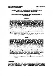
SDVRP-MDA Demands are in parentheses, the vehicle capacity is 120, and p is the minimum fraction of a customer’s demand that must be satisfied by a vehicle
SDVRP p=0
SDVRP−MDA p = .3
Total Distance = 25
Total Distance = 27
VRP Total Distance = 30
3 (80)
1
(100)
(100)
(100)
2
2
2
5 5
5
0 2
5
(60)
3
0 (60)
(20)
1
(60)
3
(80)
1
0 (20) (40)
3
. – p.10/30
Solution Procedure for SDVRP-MDA Two-stage procedure Stage 1. Find splits using the endpoint mixed integer program with minimum delivery amount constraints (EMIP-MDA) Stage 2. Clean-up routes using the enhanced record-to-record travel algorithm (ERTR)
. – p.11/30
EMIP-MDA We start with an initial VRP solution (no splits) generated by the Clarke-Wright savings procedure Since all routes meet at the depot, we look for splits near the depot Each endpoint (node adjacent to the depot) is allowed to reallocate some of its demand according to three possibilities:
. – p.12/30
EMIP-MDA 1. No change is made 2. The endpoint is removed from its current route(s) and all of its demand is reallocated to other routes 3. Some of an endpoint’s demand is removed from its current route(s) and reallocated to other routes
. – p.13/30
Endpoint moves
Move all of customer 3’s demand
Initial Routes 3
2
3
2
4
5
1
1
2
5
4
5
1
route 2
route 2 route 1
0
3
4
route 2
route 1
Move some of customer 3’s demand
route 1 0
0
. – p.14/30
MIP Formulation Objective Function Maximize total savings from endpoint reallocation Constraints Demand reallocated to a route minus the demand reallocated from the route ≤ residual capacity of the route Demand reallocated from an endpoint ≤ total demand of the endpoint
. – p.15/30
MIP Formulation If an endpoint is removed from a route, then all of its demand is reallocated If we reallocate some demand from endpoint i prior to endpoint j, then we insert i before j If we remove an endpoint from a route, we do not insert an endpoint before it or its successor If a route has only two customers, then we remove at most one of them
. – p.16/30
MIP Formulation If we reallocate some demand from an endpoint, then the total reallocated amount is nonzero If we reallocate any demand, then we must reallocate at least the minimum delivery amount If we reallocate some, but not all, of a customer’s demand, then the amount remaining must be at least the minimum delivery amount
. – p.17/30
EMIP-MDA Example Initial solution is three direct routes. EMIP-MDA optimal objective function value is 3.
SDVRP p=0
SDVRP−MDA p = .3
Total Distance = 25
Total Distance = 27
VRP Total Distance = 30
3 (80)
1
(100)
(100)
(100)
2
2
2
5 5
5
0 2
5
(60)
3
0 (60)
(20)
1
(60)
3
(80)
1
0 (20) (40)
3
. – p.18/30
ERTR Groër, Golden, Wasil (2008) VRP heuristic (no new splits) One-point move, two-point exchange, two-opt move Three-point move and OR-opt enhancement Route clean-up procedure
. – p.19/30
Test Problems Because the SDVRP-MDA is a new variant of the SDVRP, we generated test problems with good solutions that can be estimated visually We varied the customer demands in these problems in order to test EMIP-MDA + ERTR using different minimum delivery fractions We generated 21 test problems, ranging from 8 customers to 288 customers, with four different minimum delivery fractions (.1, .2, .3, and .4)
. – p.20/30
Computational Testing A problem with 32 customers; the estimated solution cost is 831.21
. – p.21/30
Computational Testing EMIP-MDA + ERTR generates a solution with a cost of 839.62; this is an increase of 1.01% from the estimated solution; p = .2
. – p.22/30
Computational Testing N = number of customers Problem
N
p = .4
p = .3
p = .2
p = .1
Estimated Solution
SD1
8
228.28
228.28
228.28
228.28
228.28
SD2
16
708.28
714.40
708.28
734.79
708.28
SD3
16
430.58
430.58
430.58
430.58
430.58
SD4
24
631.06
631.06
640.02
631.06
631.06
SD5
32
1390.57
1408.12
1390.57
1390.57
1390.57
SD6
32
831.21
831.21
839.62
852.88
831.21
SD7
40
3640.00
3714.40
3640.00
3640.00
3640.00
SD8
48
5100.00
5200.00
5068.28
5094.79
5068.28
SD9
48
2044.20
2059.84
2071.05
2137.94
2044.20
SD10
64
2704.69
2749.11
2785.01
2772.91
2684.85
SD11
80
13363.90
13612.12
13280.00
13280.00
13280.00
. – p.23/30
Computational Testing Problem
N
p = .4
p = .3
p = .2
p = .1
Estimated Solution
SD12
80
7258.92
7399.06
7279.97
7279.97
7280.00
SD13
96
10171.60
10367.06
10110.57
10110.57
10110.57
SD14
120
10780.00
11023.00
10819.29
10920.01
10920.00
SD15
144
15216.30
15271.77
15160.04
15223.42
15151.10
SD16
144
3382.16
3449.05
3497.97
3755.42
3381.32
SD17
160
26651.70
26665.76
26559.91
26559.93
26560.00
SD18
160
14357.80
14546.58
14302.22
14560.00
14380.30
SD19
192
20349.2
20559.21
20231.15
20212.84
20191.20
SD20
240
40022.70
40408.22
39739.27
39840.00
39840.00
SD21
288
11436.50
11491.67
11598.60
12445.52
11271.10
. – p.24/30
Computational Testing We tested the EMIP-MDA + ERTR on three benchmark problem sets from the literature 1. Belenguer, Martinez, and Mota (2000) 2. Archetti, Speranza, and Hertz (2006) 3. Chen, Golden, Wasil (2007) Customer demands fall into different ranges: [aQ, bQ], 0 < a < b < 1, Q = vehicle capacity
. – p.25/30
Computational Testing Percent deterioration from p = 0 case Demand Range
Number of
p = .4
p = .3
p = .2
p = .1
Problems .01 − .3
15
0.1
0.1
-0.1
0.0
.1 − .5
9
0.6
0.3
0.2
0.0
.1 − .9
8
2.0
1.1
0.4
0.4
.3 − .7
8
2.4
1.7
1.1
0.8
.6 − .9
28
8.0
4.6
3.7
0.7
. – p.26/30
Observations When p > 0, we consider how solution cost is affected by increasing the value of p Solution cost increases as p increases (what we expect) When demand is small, EMIP-MDA + ERTR finds few splits, so cost varies little as p increases When demand is large, the solution cost increases significantly with p because it becomes harder to fill vehicles with small splits
. – p.27/30
Conclusions We defined a new problem: the split delivery vehicle routing problem with minimum delivery amounts (SDVRP-MDA) We developed a two-stage heuristic for solving the SDVRP-MDA
. – p.28/30
Conclusions In the first stage, we solved an endpoint mixed integer program with minimum delivery constraints (EMIP-MDA) that finds splits In the second stage, we cleaned up the routes using an enhanced record-to-to record travel algorithm (ERTR) Computational results showed that EMIP-MDA + ERTR is effective on a wide range of problems
. – p.29/30
Future Research Questions How do we revise our procedures to solve the multi-depot SDVRP? Another layer of difficulty is added to the problem – which depots will service which customers? How do we solve the multi-depot SDVRP with minimum delivery amounts?
. – p.30/30