The Study of Trust Vector Based Trust Rating ... - Semantic Scholar

World Wide Web manuscript No. (will be inserted by the editor)

The Study of Trust Vector Based Trust Rating Aggregation in Service-Oriented Environments Lei Li · Yan Wang

Received: date / Accepted: date

Abstract In most existing studies on trust evaluation, a single trust value is aggregated from the ratings given to previous services of a service provider, to indicate his/her current trust level. Such a mechanism is useful but may not be able to depict the trust features of a service provider well under certain circumstances. Alternatively, a complete set of trust ratings can be transferred to a service client for local trust evaluation. However, this incurs a big overhead in communication, since the rating dataset is usually in large scale covering a long service history. The third option is to generate a small set of data that should represent well the large set of trust ratings of a long time period. In the literature, a trust vector approach has been proposed, with which a trust vector of three values resulting from a computed regression line can represent a set of ratings distributed within a time interval (e.g., a week or a month, etc.). However, the computed trust vector can represent the set of ratings well only if these ratings imply consistent trust trend changes and are all very close to the obtained regression line. In a more general case with trust ratings for a long service history, multiple time intervals have to be determined, within each of which a trust vector can be obtained and can represent well all the corresponding ratings. Hence, a small set of data can represent well a large set of trust ratings with well preserved trust features. This is significant for large-scale trust rating transmission, trust evaluation and trust management. In this paper, we propose one greedy and two optimal multiple time interval (MTI) analysis algorithms. We also have studied the properties of our proposed algorithms analytically and empirically. These studies can illustrate that our algorithms can return a small set of MTI to represent a large set of trust ratings and preserve well the trust features. Keywords Reputation-Based Trust · Trust Rating Aggregation · Trust Vector · Multiple Time Intervals L. Li Computing Dept Macquarie University Sydney, Australia E-mail: [email protected] Y. Wang Computing Dept Macquarie University Sydney, Australia E-mail: [email protected]

2

Lei Li, Yan Wang

1 Introduction In Service-Oriented Computing (SOC) applications, various services are provided to service clients by different service providers in a loosely-coupled environment [19, 22]. When a client looks for a service from a large set of services offered by different service providers, in addition to functionality, the reputation-based trust level of a service provider is a very important concern from the view point of the service client [11, 16, 18, 19]. It is also a critical task for the trust management authority to be responsible for maintaining the list of reputable and trustworthy services and service providers, and making these information available to service clients [22]. Conceptually, trust is the measure taken by one party on the willingness and ability of another party to act in the interest of the former party in a certain situation [13, 15]. When there are a few service providers providing the same service, the service client would like to order from the service provider with the best transaction reputation. This is particularly important when the service client has to select from unknown service providers. In general, in a trust management mechanism enabled system, service clients can provide feedback and trust ratings after transactions. Then, the trust management system can calculate the trust value based on collected ratings reflecting the quality of recent transactions, with more weights assigned to later transactions [14, 30]. The trust value can be provided to service clients by publishing it on web or responding to their requests [14, 17]. An effective and efficient trust management system is highly desirable and critical for service clients to identify potential risks, providing objective trust results and preventing huge financial loss [11]. In the literature, in most existing trust evaluation models [4, 12, 18, 28, 29, 31, 33, 35, 36], a single final trust level (FTL) is computed to reflect the general or global trust level of a service provider accumulated in a certain time period (e.g., in the latest 6 months). This FTL may be presumably taken as a prediction of trustworthiness for forthcoming transactions. Single-trust-value approaches are easily adopted in trust-oriented service comparison and selection. However, a single trust value cannot preserve the trust features well, e.g., whether and how the trust trend changes. Certainly, a full set of trust ratings can serve for this purpose, but it is usually a large dataset as it should cover a long service period. A good option is to compute a small dataset to present a large set of trust ratings and well preserve its trust features. In [14], we proposed a trust vector with three values, including final trust level (FTL), service trust trend (STT) and service performance consistency level (SPCL), to depict a set of trust ratings. In addition to FTL, the service trust trend indicates whether the service trust ratings are becoming worse or better. STT is obtained from the slope of a regression line that best fits the set of ratings {R(ti ) |R(ti ) ∈ [0, 1], ti ∈ [t1 , tn ]} distributed over a time interval [t1 , tn ]. The service performance consistency level indicates the extent to which the computed STT fits the given set of trust ratings. A computed service trust vector is meaningful only if the SPCL value is high, which indicates that all ratings distributed in the time interval are very close to the computed regression line. Given a large set of trust ratings {R(ti ) |R(ti ) ∈ [0, 1] is the rating for the service delivered at time ti }, if the trust trend changes greatly in the whole time interval [t1 , tn ] (ti ∈ [t1 , tn ]), [t1 , tn ] should be divided into multiple time intervals, each of which corresponds to a subset of ratings that can be represented by one trust vector with a high SPCL value. This task requires efficient algorithms that can determine multiple time intervals. Meanwhile, the set of computed time intervals is expected to be the minimal. For multiple time interval (MTI) analysis, in order to generate multiple trust vectors from a large set of trust ratings, we propose three MTI algorithms: the bisection-based boundary

The Study of Trust Vector Based Trust Rating Aggregation in Service-Oriented Environments

3

excluded greedy MTI algorithm, the boundary excluded optimal MTI algorithm and the boundary mixed optimal MTI algorithm. The difference between the boundary included MTI algorithm and the boundary excluded MTI algorithm is that in the computed MTI, two adjacent time intervals can or can not have common boundaries. We study the properties of our proposed algorithms both analytically and empirically. In addition, we compare these three MTI algorithms with two existing MTI algorithms in the literature, including the boundary included greedy MTI algorithm and the boundary included optimal MTI algorithm [30]. Our contributions in this paper can be briefly summarized as follows. 1. The bisection-based boundary excluded greedy MTI algorithm consumes much less CPU time than any of the other four MTI algorithms. However, it cannot guarantee returning the minimal set of MTI. 2. The boundary excluded optimal MTI algorithm can return the minimal set of boundary excluded MTI. 3. The boundary mixed optimal MTI algorithm returns a minimal set of boundary mixed MTI. This set is no larger than the set returned by any of the other four MTI algorithms. 4. With any of our proposed algorithms, a small set of data can represent well a large set of trust ratings with well preserved trust features. This paper is organized as follows. Section 2 reviews existing trust aggregation approaches and existing trust vector approaches. Section 3 introduces the service trust vector evaluation approach applied for MTI analysis algorithms. In Section 4, one greedy and two optimal multiple time interval analysis algorithms are proposed. Section 5 presents our analytical and empirical studies on the effectiveness and efficiency of our proposed algorithms. Finally Section 6 concludes our work. 2 Related Work 2.1 Trust Aggregation Approaches In Online Environments There are many trust aggregation approaches in the literature, which compute a single trust value to reflect the general trust level. We briefly review some of them proposed for different application environments. 2.1.1 Trust Evaluation in E-Commerce Environments Trust is an important issue in e-commerce (EC) environments. At eBay [1], after each transaction, a buyer can give feedback with a rating of “positive”, “neutral” or “negative” to the trust management system according to the service quality of the seller. eBay calculates the feedback score of a seller S = P − N , where P is the number of positive ratings left by P buyers and N is the number of negative ratings. The positive feedback rate R = P +N (e.g., R = 99.1%) is then calculated and displayed on web pages. This is a simple trust management system providing valuable reputation information to buyers. In [36], the Sporas system is introduced to evaluate trust for EC applications based on the ratings of transactions in a recent time period. In this method, the ratings of later transactions are given higher weights as they are more important in trust evaluation. The Histos system proposed in [36] is a more personalized reputation system compared to Sporas. Unlike Sporas, the reputation of a user in Histos depends on who makes the query, and how that

4

Lei Li, Yan Wang

person rated other users in the online community. In [27], Song et al. apply fuzzy logic to trust evaluation. Their approach divides sellers into multiple classes of reputation ranks (e.g., a 5-star seller, or a 4-star seller). In [32], Wang and Lin present some reputation-based trust evaluation mechanisms to more objectively depict the trust level of sellers on forthcoming transactions and the relationship between interacting entities.

2.1.2 Trust Evaluation in P2P Information Sharing Networks The issue of trust has been actively studied in Peer-to-Peer (P2P) information sharing networks, as in this environment a client peer needs to know prior to download actions which serving peer can provide complete files. In [4], Damiani et al. propose an approach for evaluating the reputation of peers through a distributed polling algorithm and the XRep protocol before initiating any download action. This approach adopts a binary rating system and is based on the Gnutella [2] query broadcasting method. EigenTrust [12] adopts a binary rating system as well, and aims to collect the local trust values of all peers to calculate the global trust value of a given peer. Some other earlier studies also adopted the binary rating system. In [35], Xiong et al. propose a PeerTrust model which has two main features. First, they introduce three basic trust parameters (i.e., the feedback that a requesting peer receives from other peers, the total number of transactions that a serving peer performs, the credibility of the feedback sources) and two adaptive factors in computing the trustworthiness of peers (i.e., the transaction context factor and the community context factor). Second, they define some general trust metrics and formulas to aggregate these parameters into a final trust value. In [21], Marti et al. propose a voting reputation system that collects responses from other peers on a target peer. The final reputation value is calculated by aggregating the values returned by responding peers and the requesting peer’s experience with the target peer. In [38], Zhou et al. discover a power-law distribution in peer feedbacks, and develop a reputation system with a dynamical selection on a small number of power nodes that are the most reputable in the system.

2.1.3 Trust Evaluation in Service-Oriented Environments In the literature, the issue of trust also has received much attention in the field of serviceoriented computing (SOC). In [29], Vu et al. present a model to evaluate service trust by comparing the advertised service quality and the delivered service quality. If the advertised service quality is as good as the delivered service quality, the service is reputable. In [33], Wang et al. propose some trust evaluation metrics and a formula for trust computation with which a final trust value is computed. In addition, they propose a fuzzy logic based approach for determining reputation ranks that particularly differentiates the service periods of new service providers and old (long-existing) ones. The aim is to provide incentives to new service providers and penalize those old service providers with poor service quality. In [20], Malik et al propose a set of decentralized techniques aiming at evaluating reputation-based trust with the ratings from clients to facilitate the trust-based selection and composition of Web services. In [3], Conner et al. present a trust model that allows service clients with different trust requirements to use different weight functions that place emphasis on different transaction attributes. This customized trust evaluation provides flexibility for service clients to have different trust values from the same feedback data.


5

2.1.4 Trust Evaluation in Multi-Agent Systems Trust is also an important issue in the field of multi-agent systems. In [10], Jøsang describes a framework for combining and assessing subjective ratings from different sources based on Dempster-Shafer belief theory [26]. In [28], Teacy et al. introduce the TRAVOS system (Trust and Reputation model for Agent-based Virtual OrganisationS), which calculates an agent’s trust on an interaction partner using probability theory, taking into account past interactions between agents. In [7], Griffiths proposes a multi-dimensional trust model which allows agents to model the trust of others according to various criteria. In [25], Sabater et al. propose a model discussing trust development between groups. When calculating the trust from individual A to individual B, a few factors are considered, e.g., the interaction between A and B, the evaluation of A’s group on B and B’s group, and A’s evaluation on B’s group. In [5], a community-wide trust evaluation method is proposed where the final trust value is computed by aggregating the ratings (termed as votes in [5]) and other aspects (e.g., the rater’s location and connection medium). In addition, this approach computes the trust level of an assertion (e.g., trustworthy, untrustworthy) as the aggregation of multiple fuzzy values representing the trust resulting from human interactions. In [9], in trust evaluation, the motivations of agents and the dependency relationships among them are also taken into account.

2.2 Existing Trust Vector Approaches In the literature, there exist some approaches using trust vectors, with different focuses. In [24], Ray et al. propose a trust vector that consists of the experience of a truster about a trustee, the knowledge of the truster regarding the trustee for a particular context, and the recommendation of other trustees. The focus of this model is how to address these three independent aspects of trust in evaluations. In [37], Zhao et al. propose a method using a trust vector to represent the directed link with a trust value between two peers. The trust vector includes a truster, a trustee and the trust value that the truster gives to the trustee. In [31], Wang et al. propose an approach to evaluate situational transaction trust in e-commerce environments, which binds a new transaction with the trust ratings of previous transactions. Since the situational trust vector includes service specific trust, service category trust, transaction amount category specific trust and price trust, it can deliver more objective transaction specific trust information to buyers and prevent some typical attacks. In summary, these existing approaches using trust vectors have their goals, which are totally different from that of our model.

3 Trust Vector Evaluation In cognitive science, it has been pointed out that people are motivated to maintain consistency among their actions [34]. This consistency provides the rationale that the performance of a service provider during a time interval can be consistent implying a consistent trust level. In this section, we briefly introduce our trust vector approach proposed in [14] that depicts the trust level with three values, including final trust level (FTL), service trust trend (STT) and service performance consistency level (SPCL). Hence, a trust vector can represent a large volume of trust ratings.

Lei Li, Yan Wang

Rating value

Rating value

6

Time t

Time t (b) upgoing

Rating value

Rating value

(a) coherent

Time t (c) dropping

Time t (d) uncertain

Fig. 1 Several STT cases

3.1 Final Trust Level (FTL) Evaluation The calculation of FTL follows a common principle below, which is termed as recency effect in cognitive science [34]. This principle appears in a number of studies on service trust evaluations [14, 17, 36]. Principle 1 The final trust value should be computed by taking the trust ratings in a recent time interval into account, with more weight given to the ratings of later services. Definition 1 Based on Principle 1, the FTL value for time interval [t1 , tn ] can be calculated as: Pn wt · R(ti ) [t1 ,tn ] Pn i = i=1 TFTL , (1) i=1 wti where ti ∈ [t1 , tn ] and wti can be calculated as the exponential moving average [8]: wti = αtn −ti ,

0 < α ≤ 1.

(2)

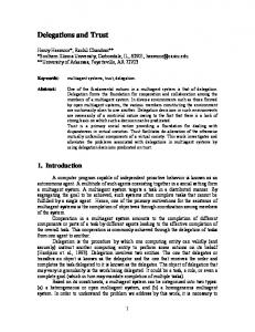
Actually, most existing single-trust-value methods (e.g., the methods proposed in [18, 33, 36]) can be adopted to compute the FTL value if they are based on non-binary ratings {R(ti ) } and follow Principle 1. 3.2 Service Trust Trend (STT) Evaluation STT aims to illustrate the trend of service trust value changes in a given time interval. Some typical cases of STT are depicted in Fig. 1, which are “coherent”, “upgoing”, “dropping” and “uncertain” in sequence. Let (t1 , R(t1 ) ), (t2 , R(t2 ) ), . . ., (tn , R(tn ) ) be the given data points within a time interval [t1 , tn ], where R(ti ) ∈ [0, 1] is the trust rating for the services delivered during a short time period ti (ti < ti+1 , t1 = tstart and tn = tend ). In general, R(ti ) can be the value aggregated from a set of ratings for the services delivered at ti (e.g., a day, or a week) [30].


7

Rating value

regression line (weighted least-squares fit)

data points

distance

Time t

Rating value

Rating value

Rating value

Fig. 2 Weighted least square linear regression

Time t

1

0

Time t

(a) absolutely consistent

Time t

(b) relatively consistent

(c) inconsistent

Fig. 3 Several SPCL cases

In order to evaluate the STT of a set of ratings {R(ti ) |ti ∈ [t1 , tn ]} for time interval [t1 , tn ], following Principle 1, we have designed a weighted least square linear regression method in [14], as depicted in Fig. 2. This method is used to obtain the best-fit straight line from a set of data points {(ti , R(ti ) )}. It is characterized by the sum of weighted squared residuals with its least value, where a residual is the distance from a data point to the regression line (see Fig. 2). Once the regression line is obtained R = a0 + a1 t,

(3)

its slope a1 is the STT value.

3.3 Service Performance Consistency Level (SPCL) Evaluation The SPCL value offers the indication of the consistency level of the service trust ratings in a certain time interval. Some typical SPCL cases are depicted in Fig. 3. [t1 ,tn ] TSPCL , the SPCL value for time interval [t1 , tn ], is a monotonically decreasing function of the weighted mean distance from rating points {(ti , R(ti ) )} to the corresponding regression line. Then, the SPCL value for time interval [t1 , tn ] can be defined by [t ,t ]

1 n TSPCL =1−2

[t ,t ]

Pn

i=1

1 n Obviously, we have TSPCL ∈ [0, 1].

wti |R(ti ) − (a0 + a1 ti )|

q

1 + a21

Pn

i=1

wti

.

(4)

Rating value

Rating value

Lei Li, Yan Wang

Rating value

8

Time t

Time t

Time t

(b) Case 2 with one time interval

(c) Case 3 with one time interval

Rating value

Rating value

Rating value

(a) Case 1 with one time interval

Time t

Time t

(d) Case 1 with two time intervals

Time t

(e) Case 2 with two time intervals

(f) Case 3 with four time intervals

Fig. 4 Several MTI examples

3.4 Service Trust Vector Based on the above introductions, we can define the service trust vector as follows. Definition 2 The service trust vector T [t1 , tn ] is T

[t1 ,tn ]

[t1 ,tn ]

[t ,tn ]

= < TFTL1

for the trust ratings given in time interval [t ,tn ]

, TSTT1

[t ,t ]

1 n , TSPCL >.

(5)

4 Multiple Time Interval (MTI) Analysis A single trust vector with three values can represent well the ratings in a given time interval [t1 , tn ] if its SPCL value is high (i.e., 0.9 or more). However, when the trust trend significantly changes in [t1 , tn ], though a single trust vector can be computed, the SPCL value will be low, indicating that the obtained trust vector or regression line can not represent all ratings precisely. In such a case, in order to represent all trust ratings well, multiple intervals in [t1 , tn ] should be determined, within each of which one trust vector with a high SPCL value can be obtained to represent the corresponding ratings well. For example, in Fig. 4, we can notice that all three cases are quite different from each other in terms of trust trend changes. If only one trust vector is computed in each case, all three cases have approximately the same TFTL , TSTT and TSPCL . However, in each case, most points have clear distances to the obtained regression line. This leads to a low SPCL value, indicating that the obtained single trust vector (or regression line) cannot represent all trust ratings well. Instead, in each case, the whole time interval can be divided into multiple time intervals (i.e., 2 time intervals in Fig. 4(d) & (e), and 4 time intervals in Fig. 4(f)). In each sub-time interval, one trust vector (or a regression line) with a high SPCL value can represent all corresponding ratings well.

1

1

0.75

0.75

Rating value

Rating value


0.5 0.25 0

0 1

3

6

0.5 0.25 0

9 Time t

0 1 2

0.75

0.75

0.25 0

6

9 Time t

(b) included boundary 1 Rating value

Rating value

(a) raw data 1

0.5

9

0.5 0.25

0 1 2 3 4 5 9 Time t (c) excluded boundaries

0

0 1

3 4 6 9 Time t (d) mixed boundaries

Fig. 5 MTI examples with different boundaries

4.1 Boundaries of MTI In order to determine multiple time intervals, we first need to study the boundaries of time intervals. For example, in Fig. 5(b), t = 1 and t = 2 are the boundaries of time interval [1, 2]. In multiple time interval analysis, there are two types of boundaries as follows. Included boundary: Two adjacent time intervals have the same boundaries. For example, in Fig. 5(b), boundary t = 2 is included in both time interval [1, 2] and time interval [2, 9]. Excluded boundary: The boundary of a time interval is excluded from adjacent time intervals. For example, in Fig. 5(c), boundary t = 2 of time interval [1, 2] is excluded from adjacent time interval [3, 4], and boundary t = 3 of time interval [3, 4] is also excluded from adjacent time interval [1, 2]. With these two types of boundaries, we can have three kinds of MTI algorithms as follows, which determine the multiple time intervals of a given set of ratings. Boundary included MTI algorithm: Adjacent time intervals determined by such an algorithm have a common boundary, i.e., the included boundary (see Fig. 5(b)). Boundary excluded MTI algorithm: Adjacent time intervals computed by such an algorithm have no common boundary, i.e., boundaries of MTI are excluded (see Fig. 5(c)). Boundary mixed MTI algorithm: Both included boundaries and excluded boundaries may appear in the adjacent time intervals computed by such an algorithm (see Fig. 5(d)). For example, there are some ratings plotted in Fig. 5(a). With a boundary included MTI algorithm, we can assume to have 2 time intervals [1, 2] and [2, 9] with included boundary,

10

Lei Li, Yan Wang

which are depicted in Fig. 5(b). In contrast, with a boundary excluded MTI algorithm, we can have 3 time intervals [1, 2], [3, 4] and [5, 9] with excluded boundaries, which are depicted in Fig. 5(c). However, with a boundary mixed MTI algorithm, we can have 3 time intervals [1, 3], [4, 6] and [6, 9], which are depicted in Fig. 5(d). Here t = 3 and t = 4 are excluded boundaries while t = 6 is an included boundary. In our previous work [30], two boundary included MTI algorithms, including the boundary included greedy MTI algorithm and the boundary included optimal MTI algorithm, have been proposed. While the boundary included greedy MTI algorithm is to include as many ratings as possible in one time interval under the condition of included boundary, the boundary included optimal MTI algorithm can return the minimal set of MTI under the same condition. In this paper, we first propose a boundary excluded greedy MTI algorithm and a boundary excluded optimal MTI algorithm for MTI analysis. Then we further develop a boundary mixed optimal MTI algorithm that can return a minimal set of MTI, which is no larger than the set returned by any of the other four algorithms. 4.2 Bisection-based Boundary Excluded Greedy MTI Algorithm [t ,t ]

1 n Take (t1 , R(t1 ) ) as the starting point and (tn , R(tn ) ) as the ending point. If TSPCL ≥ ², the (t1 ) (tn ) regression line starts from (t1 , R ) and ends at (tn , R ); otherwise, we need an MTI algorithm which can return a set of MTI. [t1 ,t] Now let us focus on the function TSPCL in Eq. (4), analyze its properties and determine the MTI. We introduce some theorems below to generalize these properties, which are also depicted in Fig. 6.

Lemma 1 ∀i ∈ [1, n − 1], [t ,t

]

i i+1 TSPCL = 1.

(6)

Proof: As there are only two data points (ti , R(ti ) ) and (ti+1 , R(ti+1 ) ) in time interval [ti , ti+1 ], both of them lie on the corresponding regression line from (ti , R(ti ) ) to (ti+1 , R(ti+1 ) ). The straight line from (ti , R(ti ) ) to (ti+1 , R(ti+1 ) ) is the regression line. Hence, [ti ,ti+1 ] following Eq. (4), we have TSPCL = 1. ¤ [t1 ,t2 ] When i = 1, following Lemma 1, we have TSPCL = 1. This confirms the fact that all [t1 ,t] the TSPCL functions (t ≥ t2 ) in Fig. 6 (b)(d)(f)(h) start from 1. Theorem 1 With 1 ≤ i < j < k ≤ n, ∀² ∈ (0, 1), if ³

[t ,t ]

i j TSPCL −²

´³

[t ,t ]

´

i k TSPCL − ² < 0,

(7)

[t ,t]

i then TSPCL = ² has at least one root in time interval [tj , tk ].

[t ,t]

i is a continuous function of variable t, according to the intermediate value Proof: As TSPCL [ti ,t] theorem in mathematical analysis [23], the condition in Eq. (7) implies that TSPCL = ² has at least one root in the interval [tj , tk ]. ¤ [t1 ,t] [t1 ,t40 ] Take the function TSPCL in Fig. 6(f) as an example. With ² = 0.9, we have TSPCL > [t1 ,t80 ] [t1 ,t40 ] [t1 ,t80 ] 0.9 and TSPCL < 0.9, i.e., (TSPCL − 0.9)(TSPCL − 0.9) < 0. In addition, we can [ti ,t] observe that TSPCL = 0.9 has a root in time interval [40, 80], which confirms Theorem 1.

Rating value

Rating value

Rating value

Rating value


1

11

1 0.9

0.5

0.8 0.7

0

1

20 40 60 80 (a) raw data in Case 1

0.6

Time t

2

40 60 80 (b) T[t , t] in Case 1

Time t

20 40 60 80 , t] (d) T[tSPCL in Case 2

Time t

20 40 60 80 , t] (f) T[tSPCL in Case 3

Time t

20

Time t

20

1

SPCL

1

1

0.9 0.8

0.5

0.7 0

1

1

20 40 60 80 (c) raw data in Case 2

0.6

Time t

2

1

1 0.9

0.5

0.8 0.7

0

1

1

20 40 60 80 (e) raw data in Case 3

0.6

Time t

2

1

1 0.9

0.5

0.8 0.7

0

1

20 40 60 80 (g) raw data in Case 4

0.6

Time t

2

(h)

40 1, t] T[tSPCL

60

80

in Case 4

[t ,t]

1 Fig. 6 The properties of SPCL function TSPCL

[t ,t ]

[t ,t]

i j i Theorem 2 With 1 ≤ i < j ≤ n, ∀² ∈ (0, 1), if TSPCL < ², then TSPCL = ² has at least one root in time interval [ti+1 , tj ].

[t ,t

[t ,t ]

]

i j i i+1 Proof: Following Lemma 1, we know TSPCL = 1 > ². In addition, with TSPCL < ², [ti ,tj ] [ti ,ti+1 ] we have (TSPCL − ²)(TSPCL − ²) < 0. Then, following Theorem 1, we can know that [ti ,t] TSPCL = ² has at least one root in time interval [ti+1 , tj ]. ¤

[t ,t]

1 In Fig. 6, with ² = 0.9, for each case we have TSPCL < 0.9. In addition, we can observe [t1 ,t] that for each case, TSPCL = 0.9 has at least one root in time interval [t1 , t100 ]. This confirms Theorem 2 empirically. Now let us introduce our bisection-based boundary excluded greedy MTI algorithm in detail. Let tlbi denote the left boundary of the ith time interval, and let trbi denote the right boundary of the ith time interval. In this algorithm, in order to determine the first time interval [tlb1 , trb1 ] (tlb1 = t1 ), we need to find the maximal right time boundary trb1 [t1 ,trb1 ] [t1 ,t] satisfying TSPCL ≥ ². If the root t∗ of TSPCL = ² can be obtained, we round down t∗ and ∗ ∗ let trb1 = bt c (e.g., if t = 63.25, then trb1 = b63.25c = 63). Then set tlb2 = trb1 +1 (i.e., if trb1 = 63, then tlb2 = 64), and repeat the above process until the last time interval reaches tn . Thus, all MTI can be determined.

12

Lei Li, Yan Wang

Algorithm 1 Bisection-based boundary excluded greedy MTI algorithm Input: trust ratings R(ti ) , the threshold ² of TSPCL (such as 0.9), the given time interval [t1 , tn ]. Output: the boundary set tb of MTI. 1: j ⇐ 1; 2: left time boundary tlbj ⇐ t1 ; 3: right time boundary trbj ⇐ tn ; [tlb ,tn ]

4: while TSPCLj < ² do 5: tleft ⇐ tlbj ; 6: tright ⇐ tn ; 7: while tright − tleft > 1 do 8: 9: 10:

tleft +tright ; 2 [tlb ,tmid ]

tmid =

if TSPCLj == λ then trbj ⇐ tmid ; [tlb ,tmid ]

11: else if TSPCLj > λ then 12: tleft ⇐ tmid ; 13: else 14: tright ⇐ tmid ; 15: end if 16: end while 17: find t∗j < tleft < tright < t∗j + 1, then let t∗j ⇐ btleft c and trbj ⇐ t∗j ; 18: j ⇐ j + 1; 19: tlbj ⇐ trbj−1 +1 ; 20: end while T T 21: return tb ⇐ [tT lb trb ] ;

[t ,t]

1 Now the task is to find the root of equation TSPCL = ². Our method is to repeatedly [t1 ,t] bisect the time interval that contains a root of TSPCL = ², until a subinterval can be selected which is smaller than 1. Let us explain this bisection process in detail with an example [t1 ,t100 ] [t1 ,t] depicted in Fig. 6(f). With ² = 0.9, as TSPCL < 0.9, according to Theorem 2, TSPCL =² has a root in time interval [t2 , t100 ]. By bisecting time interval [t2 , t100 ], with midpoint [t1 ,t51 ] [t1 ,t] t51 , we have TSPCL > 0.9. Thus, according to Theorem 1, TSPCL = ² has a root in time interval [t51 , t100 ]. By bisecting time interval [t51 , t100 ] at midpoint t75.5 , we can [t1 ,t75.5 ] [t1 ,t] obtain TSPCL < 0.9. According to Theorem 1, TSPCL = ² has a root in time interval [t1 ,t] [t51 , t75.5 ]. We repeatedly bisect the time interval containing a root of TSPCL = ², until [t1 ,t] we obtain that TSPCL = ² has a root in [t63.25 , t64.0156 ], where 64.0156 − 63.25 < 1. Hence, the right boundary of the first time interval can be determined as trb1 = tb63.25c = t63 . Now with the left boundary of the second time interval tlb2 = t64 , we can repeat the above process to determine the right boundary trb2 for the second regression line. The whole process terminates when tn is determined as the right boundary of a regression line (the last one).

The bisection-based boundary excluded greedy MTI algorithm (Algorithm 1) works as follows. Step 1: Take (t1 , R(t1 ) ) as the starting point and (tn , R(tn ) ) as the initial ending point (lines 1-3 in Algorithm 1). [t ,t ]

1 n a) If TSPCL ≥ ², the regression line starts from (t1 , R(t1 ) ) and ends at (tn , R(tn ) ) (line 4);


13

[t ,t]

1 b) otherwise, following Theorem 2, function TSPCL = ² has a root in interval [t2 , tn ]. We initialize the left boundary tleft ⇐ t1 and the right boundary tright ⇐ tn (lines 5-6). [t1 ,t] = ², and the midpoint of interval c) Time interval [tleft , tright ] contains a root of TSPCL tleft +tright [tleft , tright ] is tmid ⇐ (line 8). 2 [t1 ,tmid ] d) If TSPCL = ², the first time interval [t1 , t∗1 ] can be determined such that t∗1 < tmid < t∗1 + 1 (lines 9-10). [t1 ,tmid ] [t1 ,t] e) If TSPCL > ², TSPCL = ² has a root in the interval [tmid , tn ], and the left boundary tleft is replaced by tmid , i.e., tleft ⇐ tmid (lines 11-12); [t1 ,t] f) otherwise, TSPCL = ² has a root in the interval [t1 , tmid ], and the right boundary tright is replaced by tmid , i.e., tright ⇐ tmid (lines 13-15). g) Procedures c)-f) repeat until the first time interval [tlb1 ⇐ t1 , trb1 ⇐ t∗1 ] can be determined such that t∗1 < tleft < tright < t∗1 +1 and t∗1 ⇐ btleft c. The corresponding [t1 ,t∗ ] regression line is the longest one that starts from (t1 , R(t1 ) ) and satisfies TSPCL ≥ ² (lines 7-17). ∗ Step 2: Take (t∗1 +1, R(t1 +1) ) as the new starting point and (tn , R(tn ) ) as the ending point. The time interval [tlb2 ⇐ t∗1 + 1, trb2 ⇐ t∗2 ] (t∗2 ∈ [t∗1 + 1, tn ]) can be determined following the same procedure introduced in Step 1, and a regression line can be drawn ∗ ∗ ∗ [t∗ 1 +1,t2 ] from (t∗1 + 1, R(t1 +1) ) to (t∗2 , R(t2 ) ) satisfying TSPCL ≥ ² (lines 4-20). Step 3: Repeat Step 2 until the last regression line reaches (tn , R(tn ) ).

The computation of TSPCL incurs a complexity of O(n) (line 9), where n is the number of data points, i.e., n = |{(ti , R(ti ) )}|. As it is contained in the bisection process (O(n log n)) (lines 4-20), the bisection-based boundary excluded greedy MTI algorithm incurs a complexity of O(n2 log n). 4.3 Boundary Excluded Optimal MTI Algorithm As the above bisection-based boundary excluded greedy MTI algorithm cannot guarantee finding the minimal set of time intervals, now we develop a boundary excluded optimal MTI algorithm, which can deliver the minimal set of boundary excluded regression lines. In this optimal MTI algorithm, each point (ti , R(ti ) ) is taken as a vertex vi in a graph. [ti ,tj ] There is a directed edge from vi to vj (i < j) of weight 1 if TSPCL ≥ ². Thus, the task to obtain a minimal set of MTI is converted to the one to find the shortest path from v1 (i.e., point (t1 , R(t1 ) )) to vn (i.e., point (tn , R(tn ) )) with excluded boundaries, i.e., if there is a directed edge from vi to vj in the shortest path, the next edge in the path starts from vj+1 , not vj . For this task, we extend Dijkstra’s shortest path algorithm [6] as follows. In Dijkstra’s shortest path algorithm, when dealing with the current vertex vi , which changes unvisited to visited, we need to update the distance from v1 to every unvisited vertex with distance 1 to vi . In contrast, in boundary excluded optimal MTI algorithm, when dealing with the current vertex vi , we need to update the distance from v1 to every unvisited vertex with distance 1 to vi+1 , not vi . The obtained shortest path from v1 to vn with excluded boundaries corresponds to the minimal set of boundary excluded regression lines from (t1 , R(t1 ) ) to (tn , R(tn ) ). In this section, we introduce how our boundary excluded optimal MTI algorithm (Algorithm 2) works.

14

Lei Li, Yan Wang

Algorithm 2 Boundary Excluded Optimal MTI algorithm Input: trust ratings R(ti ) , the threshold ² of TSPCL (such as 0.9), the given time interval [t1 , tn ]. Output: the minimal boundary set vb of MTI. 1: for all i ∈ [1, vn ] do 2: for all j ∈ [i, vn ] do [i,j] 3: if TSPCL ≥ ² then 4: Mi,j ⇐ 1; 5: else 6: Mi,j ⇐ ∞; 7: end if 8: end for 9: end for 10: for all vi ∈ [v1 , vn ] do 11: dis(vi ) ⇐ Mv1 ,vi ; 12: end for 13: initialize vector unvisit ⇐ {v1 , v2 , . . . , vn }; 14: let u be v1 ; 15: while unvisit 6= ∅ do 16: let u be vi ∈ unvisit with the smallest dis(vi ); 17: remove u from unvisit; 18: for all vj with Mu+1,vj = 1 do 19: temp ⇐ dis(u) + Mu+1,vj ; 20: if temp < dis(vj ) then 21: dis(vj ) ⇐ temp; 22: previous(vj ) ⇐ u; 23: end if 24: end for 25: end while 26: vk ⇐ vn ; 27: vb ⇐ ∅; 28: while previous(vk ) 6= v1 do 29: vk ⇐ previous(vk ); 30: vb ⇐ vb ∪ vk ; 31: end while 32: return vb ;

Step 1: Take (ti , R(ti ) ) as vertex vi . Initialize the adjacent matrix M with n vertices where [ti ,tj ] the weight of the edge between vi and vj is Mi,j ⇐ 1 if TSPCL ≥ ² (i < j, i, j = 3 1, . . . , n); otherwise, Mi,j ⇐ ∞ (O(n )) (lines 1-9 in Algorithm 2). Step 2: Let dis(vi ) denote the distance from v1 to vi . Initialize the distance dis(vi ) for every vertex vi according to the adjacent matrix M (O(n)) (lines 10-12). Step 3: Mark all vertices as unvisited. Set v1 as the current vertex, and mark it as visited (O(n)) (lines 13-14). Step 4: For current vertex vi , considering all the unvisited vertices with distance 1 to its neighbors vi+1 , denoted as {vk }, compute the distance dis(vk ) respectively. If this computed dis(vk ) is less than the previous recorded dis(vk ), overwrite the recorded distance with the computed distance. If all vertices have been visited, go to Step 5. Otherwise, set the unvisited vertex vj with the smallest dis(vj ) as the current vertex vi , mark it as visited and go back to the beginning of Step 4. (O((n + m) log n), where P − − vi deg (vi ) = 2m, deg (vi ) is the indegree of vi ) (lines 15-25). Step 5: The recorded dis(vn ) is now minimized, and the corresponding path from v1 to vn is returned (lines 26-32).


15

Since n3 dominates m log n, the boundary excluded optimal MTI algorithm incurs a complexity of O(n3 ), where n is the number of data points, i.e., n = |{(ti , R(ti ) )}|.

4.4 Boundary Mixed Optimal MTI Algorithm Our empirical studies can demonstrate that both the boundary included optimal MTI algorithm [30] and the boundary excluded optimal MTI algorithm can return the minimal set of MTI with constraints, namely, the boundaries are included or excluded in adjacent time intervals respectively. If there is no such constraint, there may exist a set of boundary mixed time intervals, which is no larger than the set returned by either the boundary included optimal MTI algorithm or the boundary excluded optimal MTI algorithm. This requires the use of a boundary mixed optimal MTI algorithm. Let us briefly illustrate the difference between the boundary excluded optimal MTI algorithm and the boundary mixed optimal MTI algorithm. 1. In the boundary excluded optimal MTI algorithm, when dealing with the current vertex vi , we need to update the distance from v1 to every unvisited vertex with distance 1 to vi+1 . 2. In contrast, in the boundary mixed optimal MTI algorithm, when dealing with the current vertex vi , we need to update the distance from v1 to every unvisited vertex with distance 1 to vi or vi+1 . The boundary mixed optimal MTI algorithm (Algorithm 3) works as follows. Step 1: Take (ti , R(ti ) ) as vertex vi . Initialize the adjacent matrix M with n vertices where [ti ,tj ] the weight of the edge between vi and vj is Mi,j ⇐ 1 if TSPCL ≥ ² (i < j, i, j = 3 1, . . . , n); otherwise, Mi,j ⇐ ∞ (O(n )) (lines 1-9 in Algorithm 3). Step 2: Let dis(vi ) denote the distance from v1 to vi . Initialize the distance dis(vi ) for every vertex vi according to the adjacent matrix M (O(n)) (lines 10-12). Step 3: Mark all vertices as unvisited. Set v1 as the current vertex, and mark it as visited (O(n)) (lines 13-14). Step 4: For current vertex vi , considering all the unvisited vertices with distance 1 to its neighbor vi+1 or itself vi , denoted as {vk }, compute the distance dis(vk ) respectively. If this computed dis(vk ) is less than the previous recorded dis(vk ), overwrite the recorded distance with the computed distance. If all vertices have been visited, go to Step 5. Otherwise, set the unvisited vertex vj with the smallest dis(vj ) as the current vertex P vi , mark it as visited and go back to the beginning of Step 4. (O((n + m) log n), where vi deg− (vi ) = 2m, deg− (vi ) is the indegree of vi ) (lines 15-30). Step 5: The recorded dis(vn ) is now minimized, and the corresponding path from v1 to vn is returned (lines 31-39). Since n3 dominates m log n, the boundary mixed optimal MTI algorithm incurs a complexity of O(n3 ), where n is the number of data points, i.e., n = |{(ti , R(ti ) )}|. Theorem 3 The boundary mixed optimal MTI algorithm returns the minimal set of boundary mixed time intervals. Proof: Let D(vi , vj ) denote the distance from vi to vj . In the boundary mixed optimal MTI algorithm, the following two conditions hold.

16

Lei Li, Yan Wang

Algorithm 3 Boundary Mixed Optimal MTI algorithm Input: trust ratings R(ti ) , the threshold ² of TSPCL (such as 0.9), the given time interval [t1 , tn ]. Output: the minimal boundary set vb of MTI. 1: for all i ∈ [1, vn ] do 2: for all j ∈ [i, vn ] do [i,j] 3: if TSPCL ≥ ² then 4: Mi,j ⇐ 1; 5: else 6: Mi,j ⇐ ∞; 7: end if 8: end for 9: end for 10: for all vi ∈ [v1 , vn ] do 11: dis(vi ) ⇐ Mv1 ,vi ; 12: end for 13: initialize vector unvisit ⇐ {v1 , v2 , . . . , vn }; 14: let u be v1 ; 15: while unvisit 6= ∅ do 16: let u be vi ∈ unvisit with smallest dis(vi ); 17: remove u from unvisit; 18: for all vj with Mu,vj = 1 or Mu+1,vj = 1 do 19: temp ⇐ min{dis(u), dis(u) + Mu,vj , dis(u) + Mu+1,vj }; 20: if (temp == dis(u) + Mu+1,vj )&(temp < dis(u)) then 21: dis(u) ⇐ temp; 22: previous1,vj ⇐ u; 23: previous2,vj ⇐ u + 1; 24: else if (temp == dis(u) + Mu,vj )&(temp < dis(u)) then 25: dis(u) ⇐ temp; 26: previous1,vj ⇐ u; 27: previous2,vj ⇐ u; 28: end if 29: end for 30: end while 31: vk ⇐ vn ; 32: v1,b ⇐ v1 ; 33: v2,b ⇐ vn ; 34: while previous1,vk 6= v1 do 35: v2,b ⇐ previous1,vk ∪ v2,b ; 36: vk ⇐ previous1,vk ; 37: v1,b ⇐ v1,b ∪ vk ; 38: end while T T ]T ; 39: return vb ⇐ [v1,b v2,b

[t ,t ]

i j C1: the directed edge from vi to vj (i < j) weights 1 only if TSPCL ≥ ², i.e., D(vi , vj ) = 1; otherwise it weights infinite, i.e., D(vi , vj ) = ∞. C2: if there is a directed edge from vi to vj in the shortest path, (a) with included boundary, the next edge in the path starts from vj , and D(vj , vj ) = 0. (b) with excluded boundary, the next edge in the path starts from vj+1 , not vj , and D(vj , vj+1 ) = 0.

With these distances, in the boundary mixed optimal MTI algorithm, D(v1 , vn ) is obtained from Dijkstra’s shortest path algorithm. Then D(v1 , vn ) is the minimal length which corresponds to the shortest path from v1 to vn . According to C1 & C2, a path from from v1 to vn corresponds to a set of regression lines from v1 to vn , i.e., a set of boundary mixed


17

MTI. Hence, the boundary mixed optimal MTI algorithm returns the minimal set of boundary mixed MTI, and the number of MTI is D(v1 , vn ). ¤ Similar to Theorem 3, we can prove that our proposed boundary excluded optimal MTI algorithm returns the minimal set of boundary excluded MTI. Theorem 4 The boundary mixed optimal MTI algorithm returns a set of MTI which is no larger than the set returned by either the boundary included optimal MTI algorithm or the boundary excluded optimal MTI algorithm. Proof: In the boundary included optimal MTI algorithm, for vertex vi , we need to update the distance from v1 to every unvisited vertex (e.g., vj ) with distance 1 to vi . The distance (1) from v1 to vj is denoted as dvj , and (1) (1) d(1) vj = min{dvj , dvi + 1}.

(8)

In contrast, in the boundary excluded optimal MTI algorithm, the distance from v1 to vj is (2) denoted as dvj , and (2) (2) d(2) vj = min{dvj , dvi+1 + 1}.

(9)

However, in the boundary mixed optimal MTI algorithm, the distance from v1 to vj is de(3) noted as dvj , and (3) (3) (3) d(3) vj = min{dvj , dvi + 1, dvi+1 + 1}.

(10)

Obviously, every time when updating the distance from v1 to vj , we can obtain that (1) (3) (2) d(3) vj ≤ dvj and dvj ≤ dvj .

(11)

(1) (3) (2) d(3) vn ≤ dvn and dvn ≤ dvn .

(12)

Then, we have The boundary mixed optimal MTI algorithm returns a set of time intervals that is no larger than the one returned by any of the other two optimal MTI algorithms. ¤ Theorem 4 is also confirmed empirically by Experiments 2 & 3 introduced in Sections 5.2 and 5.3.

5 Experiments In this section, we introduce the results of our experiments conducted on both a real-world dataset and synthetic datasets. The aim of our experiments is to study the effectiveness and efficiency of our proposed MTI algorithms.

5.1 Experiment 1 – Comparison of Our Single Trust Vector Approach and A Single-Trust-Value Method As pointed out in Section 3.1, the evaluation of FTL can be based on any existing singletrust-value method. In this experiment, we aim to illustrate why the service trust vector is necessary by comparing our trust vector approach with the single-trust-value method in [18], which is also based on non-binary ratings and applies to service-oriented environments.

Lei Li, Yan Wang

1

Rating value

Rating value

18

0.5 0

0

50

100 Time t

1 0.5 0

0

Rating value

Rating value

1 0.5

0

50

1 0.5 0

100 Time t

0

Rating value

Rating value

0.5

50

100 Time t

1 0.5 0

0

50

100 Time t

(f) P

(e) P5

6

Fig. 7 Trust vectors in Experiment 1 Table 1 Trust vectors in Experiment 1 P1 P2 P3 P4 P5 P6

100 Time t 4

1

0

50 (d) P

(c) P3

0

100 Time t

(b) P2

(a) P1

0

50

TFTL 0.6018 0.6013 0.6010 0.6010 0.6017 0.6012

TSTT 0.0041 0.0041 0.0001 0.0001 -0.0022 -0.0022

TSPCL 0.9574 0.8852 0.9537 0.9106 0.9517 0.9049

0.9

Rating value

Rating value


0.8 0.7 0.6 0.5

0

50

100

Rating value

Rating value

0.7 0.6

0.8 0.7 0.6 Time t 0 50 100 (b) ε=0.925 (boundary included greedy MTI algorithm)

(a) ε=0.9

0.8

0.9

0.5

Time t

0.9

19

0.9 0.8 0.7 0.6

0.5 Time t 0 50 100 0 50 100 Time t (c) ε=0.925 (bisection−based boundary excluded MTI algorithm) (d) ε=0.925 (boundary included optimal MTI algorithm) 0.9

Rating value

Rating value

0.5

0.8 0.7 0.6 0.5

0

50

100

Time t

(e) ε=0.925 (boundary excluded optimal MTI algorithm)

0.9 0.8 0.7 0.6 0.5

0

50

100

Time t

(f) ε=0.925 (boundary mixed optimal MTI algorithm)

Fig. 8 MTI in Experiment 2

In the comparison, we evaluate the trust level of six service providers P1 to P6 , with the parameter α = 1 and the weights determined by Eq. (2). Both the trust ratings and corresponding regression lines are plotted in Fig. 7. The computed trust vectors are listed in Table 1. According to Table 1, all six service providers P1 to P6 (see Fig. 7(a)-(f)) have almost the same TFTL . Therefore, they seemingly have the same trust level. However, they have different TSTT or TSPCL . In detail, P1 and P2 have the same TSTT (“upgoing”), but different TSPCL ; similarly, P3 and P4 have the same TSTT (“coherent”) but different TSPCL ; P5 and P6 have the same TSTT (“dropping”) but different TSPCL . Without calculated trust vectors, we cannot distinguish these six service providers. From this experiment, we can see that under some circumstances a service trust vector can depict the trust level more precisely than a single trust value. Hence, the introduction of the trust vector is necessary.

5.2 Experiment 2 – Comparison on the Number of Returned MTI In this experiment, we study our proposed three MTI algorithms (i.e., Algorithms 1-3 listed in Table 2) over a large set of ratings of one seller obtained from eBay [1], and compare these algorithms with two existing MTI algorithms, including the boundary included greedy

Lei Li, Yan Wang

Rating value

Rating value

Rating value

Rating value

Rating value

20

0.9 0.8 0.7

Time t

0

20 40 60 80 100 120 (a) ε=0.94 (boundary included greedy MTI algorithm) (11 time intervals)

0

20 40 60 80 100 120 Time t (b) ε=0.94 (bisection−based boundary excluded greedy MTI algorithm) (11 time intervals)

0.9 0.8 0.7

0.9 0.8 0.7

0

20 40 60 80 100 120 (c) ε=0.94 (boundary included optimal MTI algorithm) (10 time intervals)

Time t

0

20 40 60 80 100 120 (d) ε=0.94 (boundary excluded optimal MTI algorithm) (8 time intervals)

Time t

0

20 40 60 80 100 120 (e) ε=0.94 (boundary mixed optimal MTI algorithm) (7 time intervals)

Time t

0.9 0.8 0.7

0.9 0.8 0.7

Fig. 9 Comparison of five MTI algorithms in Experiment 2 Table 2 MTI algorithms compared in Experiments Algorithm 1 Algorithm 2 Algorithm 3 Algorithm 4 Algorithm 5

The bisection-based boundary excluded greedy MTI algorithm The boundary excluded optimal MTI algorithm The boundary mixed optimal MTI algorithm The boundary included greedy MTI algorithm [30] The boundary included optimal MTI algorithm [30]

MTI algorithm and the boundary included optimal MTI algorithm proposed in [30] (i.e., Algorithms 4 & 5 listed in Table 2). In the rating sample of an eBay seller, there are 11752 ratings in total about the transactions, which happened in 131 days from 13 February 2009 to 23 June 2009. At eBay, a rating can be 1 (“positive”), 0 (“neutral”) or −1 (“negative”). Like the method adopted P −N in [35], the feedback score percentage is introduced and calculated as Sp = P +N e+N , where P , N e and N are the numbers of positive, neutral and negative ratings respectively. We use each day’s ratings to compute the feedback score rate Sp , which is taken as the rating R(ti ) for time period ti (i.e., ti is a day in this case and i ∈ [1, 131]). All rating {(ti , R(ti ) )|1 ≤ i ≤ 131} are plotted in Fig. 8(a). From Figs 8 & 9, we can observe that 1. when the threshold of TSPCL is ² = 0.9, as plotted in Fig. 8(a), with any of the five MTI algorithms listed in Table 2, only 1 trust vector is obtained for the whole time interval [t1 , t131 ].

1

1

0.8

0.8

Rating value

Rating value


0.6 0.4 0.2 0

0

200

0.6 0.4 0.2 0

400 Time t

0

0.8

0.8

Rating value

Rating value

1

0.4 0.2 0

0

200

400 Time t

(b) ε=0.85 (2 time intervals)

(a) raw data 1

0.6

21

200 400 Time t (c) ε=0.87 (2 time intervals)

0.6 0.4 0.2 0

0

200 400 Time t (d) ε=0.9 (3 time intervals)

Fig. 10 Case 1 in Experiment 3 with the boundary mixed optimal MTI algorithm

2. with a higher threshold ² = 0.925, 2 time intervals are obtained by using any of the five MTI algorithms listed in Table 2. The results of Algorithms 1-5 are plotted in Fig. 8(b)(c)(d)(e)(f) respectively. 3. with a further higher threshold ² = 0.94, we can also observe from Fig. 9 that both the boundary included greedy MTI algorithm and the bisection-based boundary excluded greedy MTI algorithm return 11 time intervals (see Fig. 9(a)(b)); while the boundary included optimal MTI algorithm returns 10 time intervals (see Fig. 9(c)); the boundary excluded optimal MTI algorithm returns 8 time intervals (see Fig. 9(d)); in contrast, the boundary mixed optimal MTI algorithm returns 7 time intervals (see Fig. 9(e)). Based on the above results, among all five MTI algorithms listed in Table 2, we can observe that the boundary mixed optimal MTI algorithm can return a set of MTI which is no larger than any set returned by other algorithms. This confirms Theorem 4 empirically. 5.3 Experiment 3 – Comparison on Efficiency In this experiment, we use large-scale synthetic rating datasets to compare the efficiency of our proposed bisection-based boundary excluded greedy MTI algorithm (i.e., Algorithm 1 listed in Table 2) and two optimal MTI algorithms (i.e., Algorithms 2 & 3 listed in Table 2) with two existing MTI algorithms in [30] (i.e., Algorithms 4 & 5 listed in Table 2). We conducted our experiments on top of Matlab 7.6.0.324 (R2008a) running on a Dell Vostro V1310 laptop with an Intel Core 2 Duo T5870 2.00GHz CPU and 3GB RAM. Each result of the consumed CPU time is the average of three independent executions with very minor differences in time.

Lei Li, Yan Wang

1

1

0.8

0.8

Rating value

Rating value

22

0.6 0.4 0.2 0

0.6 0.4 0.2

0

200

400 Time t

0

0

200 400 Time t (b) ε=0.85 (6 time intervals)

0


1

0.8

0.8

Rating value

Rating value

(a) raw data 1

0.6 0.4 0.2 0

0.6 0.4 0.2

0


0

Fig. 11 Case 2 in Experiment 3 with the boundary mixed optimal MTI algorithm

In this experiment, three different sets of ratings have been used, which are plotted in Fig. 10(a) (Case 1), Fig. 11(a) (Case 2) and Fig. 12(a) (Case 3) respectively. Each dataset consists of 500 trust ratings distributed in 500 time periods (i.e., ti ∈ [t1 , t500 ]). By applying the boundary mixed optimal MTI algorithm to each case, we have the following results. Case 1: In this case (see Fig. 10(a)), with the threshold of TSPCL set as ² = 0.85, 0.87 or 0.9 respectively, we can obtain 2 or 3 time intervals as plotted in Fig. 10(b)(c)(d). Case 2: As the trust trend changes a little more frequently in this case (see Fig. 11(a)), when the threshold is set as ² = 0.85, 0.87 or 0.9 respectively, 6, 8 or 9 time intervals are obtained (see Fig. 11(b)(c)(d)). Case 3: In contrast, in Case 3 (see Fig. 12(a)), the trust trend changes the most frequently in all three cases. With the same thresholds ² = 0.85, 0.87 or 0.9, there are 13 (see Fig. 12(b)), 16 (see Fig. 12(c)) or 20 time intervals (see Fig. 12(d)) obtained respectively. Thus, in all three cases, with threshold ² = 0.85, we can use 2, 6 or 13 trust vectors respectively to approximately represent 500 trust ratings. With a high threshold ² = 0.9, we can use 3, 9 or 20 trust vectors respectively to approximately represent 500 trust ratings. Thus, with our proposed algorithms, a small set of values can represent a large set of trust ratings with well preserved trust features. In addition, in all three cases using different thresholds, we can compare the consumed CPU time of the five MTI algorithms listed in Table 2. From the results listed in Table 3, we can derive the following conclusions. Comparison of different algorithms on efficiency and the number of returned MTI:

1

1

0.8

0.8

Rating value

Rating value


0.6 0.4 0.2

0.6 0.4 0.2

0

200 (a) raw data

400 Time t

0

1

1

0.8

0.8

Rating value

Rating value

0

0.6 0.4 0.2 0

23

0

200 400 Time t (b) ε=0.85 (13 time intervals)

0


0.6 0.4 0.2

0


0

Fig. 12 Case 3 in Experiment 3 with the boundary mixed optimal MTI algorithm Table 3 Consumed CPU time in seconds and the number of returned MTI in Experiment 3

Case 6

Case 5

Case 4

Case 3

Case 2

Case 1

² 0.85 0.87 0.9 1 0.85 0.87 0.9 1 0.85 0.87 0.9 1 0.85 0.87 0.9 1 0.85 0.87 0.9 1 0.85 0.87 0.9 1

Boundary included Bisection-based greedy boundary excluded MTI algorithm greedy MTI algorithm time (s) num time (s) num 3.7 3 0.3 2 4.4 3 0.2 2 9.9 4 0.3 3 1288.9 499 8.0 250 15.6 7 0.4 6 24.2 10 0.5 8 26 10 0.5 9 1265.4 499 8.0 250 37.4 15 0.6 13 47.8 20 0.7 18 55.4 21 0.8 20 1270.7 499 8.0 250 4.2 2 0.5 2 23.7 3 0.7 3 29.3 3 0.6 3 10336 499 32.0 250 61.4 5 0.8 5 78.5 8 1.0 8 109.4 9 1 9 10289 499 31.8 250 171.5 14 1.3 14 208.7 19 1.6 19 222.1 20 1.6 20 10406 499 31.9 250

Boundary included optimal MTI algorithm time (s) num Step1 Steps2-5 Total 1296.3 1.4 1297.7 2 1299.1 1.4 1300.5 2 1296.2 1.4 1297.6 3 1301 1.6 1302.6 499 1297.3 1.5 1298.8 6 1298.4 1.4 1299.8 9 1296.6 1.4 1298 9 1299.4 1.6 1301 499 1296.4 1.5 1297.9 14 1299.1 1.5 1300.6 19 1298.2 1.5 1299.7 20 1298.4 1.6 1300 499 10473 6.2 10479 2 10467 6.1 10473 3 10472 6.2 10478 3 10507 6.2 10513 499 10474 6.2 10480 5 10500 6.6 10507 8 10494 6.3 10500 9 10493 6.2 10499 499 10481 6.1 10487 14 10491 6.2 10497 19 10472 6.4 10478 20 10509 6.3 10515 499

Boundary excluded optimal MTI algorithm time (s) Step1 Steps2-5 Total 1295.1 4 1299.1 1297.8 3.9 1301.7 1298.4 3.9 1302.3 1289 4 1293 1297.6 4 1301.6 1296.9 3.9 1300.8 1299.6 3.9 1303.5 1286.7 4 1290.7 1297.8 3.9 1301.7 1296.1 3.9 1300 1301.1 3.9 1305 1286.6 4 1290.6 10474 16.5 10491 10434 16.3 10450 10478 16.6 10495 10473 16.3 10489 10481 16.4 10497 10487 16.4 10503 10502 16.3 10526 10495 16.3 10511 10509 16.4 10525 10488 16.9 10505 10481 16.4 10497 10512 16.4 10528

num 2 2 3 250 6 8 9 250 13 16 20 250 2 3 3 250 5 8 9 250 14 19 20 250

Boundary mixed optimal MTI algorithm time (s) num Step1 Steps2-5 Total 1296.1 5.5 1301.6 2 1296.8 5.5 1302.3 2 1300.9 5.5 1306.4 3 1289.6 5.5 1295.1 250 1294.7 5.5 1300.2 6 1296.8 5.5 1302.3 8 1305.3 5.6 1310.9 9 1288.8 5.5 1294.3 250 1294.6 5.5 1300.1 13 1301.8 5.5 1307.3 16 1302.6 5.5 1308.1 20 1290 5.5 1295.5 250 10490 23.0 10513 2 10485 22.9 10508 3 10463 22.8 10486 3 10487 22.7 10510 250 10483 22.8 10506 5 10462 22.9 10485 8 10490 22.8 10513 9 10497 22.7 10520 250 10505 22.7 10527 14 10505 22.7 10528 19 10474 22.6 10497 20 10509 22.6 10532 250

24

Lei Li, Yan Wang

1. The consumed CPU time of the bisection-based boundary excluded greedy MTI algorithm is only 0.6%-8.1% of that of the boundary included greedy MTI algorithm. In addition, the former algorithm returns a set of MTI which is no larger than that returned by the latter algorithm. Hence, the bisection-based boundary excluded greedy MTI algorithm outperforms the boundary included greedy MTI algorithm in terms of efficiency. 2. The bisection-based boundary excluded greedy MTI algorithm consumes less than 0.6% of the CPU time consumed by any of the three optimal MTI algorithms. Thus, we can conclude that the bisection-based boundary excluded greedy MTI algorithm runs much faster than any of the three optimal MTI algorithms. 3. For each of the three optimal MTI algorithms, we can divide the whole algorithm into two parts, including the generation of the adjacency matrix (Step 1 introduced in Section 4.3 or Section 4.4), and the Dijkstra’s algorithm based MTI analysis (Steps 2-5). As listed in Table 3, the former part takes above 99.6% of the total consumed 2 CPU time since it has to check if TSPCL ≥ ² for all n2 − n possible edges, while the latter part takes less than 0.4% of the total consumed CPU time. 4. With the three optimal MTI algorithms, the shortest consumed CPU time is only 1.5% less than the longest one. Hence, no matter which of the three cases and with what threshold ² is used (e.g., 0.85, 0.87, 0.9 or 1), all three optimal MTI algorithms consume almost the same CPU time. 5. The boundary mixed optimal MTI algorithm returns a set of MTI which is no larger than the set returned by any of the other four MTI algorithms. This again confirms Theorem 4 empirically. Comparison on efficiency and the number of returned MTI in different cases: 1. From Case 1 to Case 3 (see Fig. 10(a), Fig. 11(a) and Fig. 12(a)), the trust trend changes more and more frequently. With the same MTI algorithm and the same threshold, this change leads to a larger set of MTI. For example, from Case 1 to Case 3, with threshold ² = 0.9, the boundary mixed optimal MTI algorithm returns 3, 9 and 20 time intervals respectively. 2. From Case 1 to Case 3, when the trust trend changes more and more frequently, with the same threshold the bisection-based boundary excluded greedy MTI algorithm needs more and more CPU time to determine the set of MTI. For example, from Case 1 to Case 3, with threshold ² = 0.9, this algorithm consumes 0.3, 0.5, and 0.8 seconds of CPU time respectively. Comparison on efficiency and the number of returned MTI with different thresholds: 1. When threshold ² becomes higher, with the same algorithm, a larger set of MTI is returned. 2. When ² becomes higher, the bisection-based boundary excluded greedy MTI algorithm consumes more CPU time. However, even with the highest threshold ² = 1, its consumed CPU time is still around 0.6% of that consumed by any of the three optimal MTI algorithms. Moreover, by applying the five MTI algorithms to larger synthetic rating datasets with 1000 ratings each (i.e. Case 4, Case 5 and Case 6) depicted in Fig. 13, we can obtain similar conclusions as introduced above in the comparison of five MTI algorithms on algorithm efficiency. In addition, from the obtained results listed in Table 3, we can see that the execution time of any of the three optimal MTI algorithms for 1000 ratings is approximately eight

1

1

0.8

0.8

0.8

0.6 0.4 0.2 0

Rating value

1

Rating value

Rating value


0.6 0.4 0.2

0

500 (a) Case 4

1000 Time t

0

25

0.6 0.4 0.2

0

500 (b) Case 5

1000 Time t

0

0

500 (c) Case 6

1000 Time t

Fig. 13 Case 4, Case 5 and Case 6 in Experiment 3

times as much as that for 500 ratings. As the datasets of 1000 ratings double those of 500 ratings in size, this confirms that the complexity of each of the three optimal MTI algorithms is O(n3 ). Therefore, by incorporating the results in Experiment 2, we can see that the bisectionbased boundary excluded greedy MTI algorithm is useful when processing large-scale rating data, because it consumes much less CPU time than any of the other four MTI algorithms. However, it cannot guarantee returning the minimal set of MTI. In contrast, the boundary mixed optimal MTI algorithm can return the smallest set of MTI among all five MTI algorithms, but it consumes much more CPU time than the two greedy algorithms. 5.4 Experiment 4 – Comparison on MTI Goodness-of-Fit With our proposed MTI algorithms, a small set of MTI can represent a large set of trust ratings well. However, how well have the trust features been preserved? Now we compare the final trust value aggregated from a set of MTI with the final trust value aggregated from trust ratings directly to see how well the trust features are preserved. In this section, prior to presenting the detailed analysis, we must first introduce the definition of the final trust value aggregated from a set of MTI. Definition 3 With a set of MTI covering the ratings {(ti , R(ti ) )} in time interval [t1 , tn ] {[tlbi , trbi ]|1 ≤ i ≤ h, tlb1 = t1 , trbh = tn },

(13)

the final trust value aggregated from the set of MTI is Ph

TeFTL ({[tlbi , trbi ]}) =

i=1

[tlb ,trbi ]

TFTL i

Pn

Prbi

k=lbi

k=1 wtk

wtk

,

(14)

where wtk is defined in Eq. (2) of Definition 1. Now we introduce the definition of MTI goodness-of-fit, which is measured from the relative difference between the final trust value aggregated from a set of MTI according to Definition 3, and the final trust value aggregated from trust ratings directly according to Definition 1. This measurement indicates how well the trust features are preserved by the set of MTI. A high goodness-of-fit of the set of MTI indicates the high effectiveness of the corresponding MTI algorithm.

26

Lei Li, Yan Wang

Definition 4 With a set of MTI covering the ratings {(ti , R(ti ) )} in time interval [t1 , tn ] {[tlbi , trbi ]|1 ≤ i ≤ h, tlb1 = t1 , trbh = tn },

(15)

the MTI goodness-of-fit is [t ,tn ]

GMTI ({[tlbi , trbi ]}) = 1 − [t ,tn ]

where TFTL1

− TeFTL ({[tlbi , trbi ]})|

|TFTL1

[t ,tn ]

TFTL1

,

(16)

is defined in Definition 1 and TeFTL ({[tlbi , trbi ]}) is defined in Definition 3.

With Definition 4, we can study the goodness-of-fit of the set of MTI returned by each of two boundary excluded MTI algorithms, including both the bisection-based boundary excluded greedy MTI algorithm and the boundary excluded optimal MTI algorithm. Theorem 5 The goodness-of-fit of the set of MTI returned by either the bisection-based boundary excluded greedy MTI algorithm or the boundary excluded optimal MTI algorithm is 100%. Proof: Let {[tlbi , trbi ]|1 ≤ i ≤ h, tlb1 = t1 , trbh = tn }

(17)

denote a set of MTI returned by either the bisection-based boundary excluded greedy MTI algorithm or the boundary excluded optimal MTI algorithm. As the set of MTI is boundary excluded, we have trbj−1 +1 = tlbj for j ∈ [2, h]. (18) By substituting Eq. (18) into Eq. (17), we then have {[trbi−1 +1 , trbi ]|1 ≤ i ≤ h, trb0 +1 = t1 , trbh = tn }. [trb

For time interval [trbi−1 +1 , trbi ], according to the definition of TFTL i−1 (1), we have Prbi (tk ) [trbi−1 +1 ,trbi ] k=rbi−1 +1 wtk R = TFTL , Prbi k=rbi−1 +1 wtk

(19) +1 ,trbi ]

in Eq. (20)

i.e., [trb

TFTL i−1

rbi X

+1 ,trbi ]

rbi X

wt k =

k=rbi−1 +1

wtk R(tk ) .

(21)

k=rbi−1 +1

For all time intervals {[trbi−1 +1 , trbi ]|1 ≤ i ≤ h} in [t1 , tn ], we have h X i=1

[trb

TFTL i−1

rbi X

+1 ,trbi ]

wt k =

rbi X

h X

wtk R(tk )

i=1 k=rbi−1 +1

k=rbi−1 +1

=

n X

wtk R(tk ) .

(22)

k=1 [t ,tn ]

According to the definition of TFTL1 [t ,tn ]

TFTL1

=

in Eq. (1), we have

Pn wt R(tk ) k=1 Pn k . k=1

wt k

(23)


27

If we now substitute Eq. (22) into Eq. (23), we then have Ph [t ,t ] TFTL1 n

=

[trb

i=1

TFTL i−1

+1 ,trbi ]

Prbi

k=rbi−1 +1

Pn

wt k

k=1 wtk

.

(24)

By substituting Eq. (24) into Eq. (14) in Definition 3, we have [t ,tn ]

TeFTL ({[trbi−1 +1 , trbi ]}) = TFTL1

.

(25)

Therefore, according to Eq. (16) in Definition 4, we can obtain that the goodness-of-fit of the set of boundary excluded MTI {[trbi−1 +1 , trbi ]} is [t ,tn ]

GMTI ({[trbi−1 +1 , trbi ]}) = 1 −

|TFTL1

− TeFTL ({[trbi−1 +1 , trbi ]})| [t ,tn ]

TFTL1

= 100%.

(26) ¤

Next, with Definition 4, we can also study the goodness-of-fit of the set of MTI returned by each of two boundary included MTI algorithms, including both the boundary included greedy MTI algorithm and the boundary included optimal MTI algorithm. Theorem 6 The goodness-of-fit of the set of MTI returned by either the boundary included greedy MTI algorithm or the boundary included optimal MTI algorithm is less than 100%. Proof: Let {[tlbi , trbi ]|1 ≤ i ≤ h, tlb1 = t1 , trbh = tn }

(27)

denote a set of MTI returned by either the boundary included greedy MTI algorithm or the boundary included optimal MTI algorithm. As the set of MTI is boundary included, we have trbj−1 = tlbj for j ∈ [2, h].

(28)

By substituting Eq. (28) into Eq. (27), we then have {[trbi−1 , trbi ]|1 ≤ i ≤ h, trb0 = t1 , trbh = tn }. [trb

For time interval [trbi−1 , trbi ], according to the definition of TFTL i−1 have Prbi (tk ) [trbi−1 ,trbi ] k=rbi−1 wtk R = TFTL , Prbi k=rbi−1 wtk

(29) ,trbi ]

in Eq. (1), we (30)

i.e., [trb

TFTL i−1

,trbi ]

rbi X

wt k =

k=rbi−1

rbi X

wtk R(tk ) .

(31)

k=rbi−1

For all time intervals {[trbi−1 , trbi ]|1 ≤ i ≤ h} in [t1 , tn ], we have h X i=1

[trb

TFTL i−1

,trbi ]

rbi X k=rbi−1

wt k =

h X

rbi X

i=1 k=rbi−1

wtk R(tk ) .

(32)

28

Lei Li, Yan Wang

As in Eq. (22) rbi X

h X

wtk R(tk ) =

i=1 k=rbi−1 +1

n X

wtk R(tk ) ,

(33)

k=1

we have rbi X

h X

wtk R(tk ) >

i=1 k=rbi−1

n X

wtk R(tk ) .

(34)

k=1

Then, by substituting Eq. (32) into Eq. (34), we have h X

[trb

TFTL i−1

rbi X

,trbi ]

i=1

n X

wtk >

k=rbi−1

wtk R(tk ) ,

(35)

k=1

i.e., Ph

i=1

[trb

TFTL i−1

,trbi ]

Prbi

k=rbi−1

Pn

k=1

wt k [t ,tn ]

According to the definitions of TFTL1 from Eq. (36) we have

wtk

>

Pn wt R(tk ) k=1 Pn k . k=1

wt k

(36)

in Eq. (1) and TeFTL ({[trbi−1 , trbi ]}) in Eq. (14), [t ,tn ]

TeFTL ({[trbi−1 , trbi ]}) > TFTL1

,

(37)

i.e., [t ,tn ]

|TFTL1

− TeFTL ({[trbi−1 , trbi ]})| > 0.

(38)

Therefore, according to Eq. (16) in Definition 4, we can obtain that the goodness-of-fit of the set of boundary included MTI {[trbi−1 , trbi ]} is [t ,tn ]

GMTI ({[trbi−1 , trbi ]}) = 1 −

|TFTL1

− TeFTL ({[trbi−1 , trbi ]})| [t ,tn ]

TFTL1

< 100%.

(39) ¤

By applying Definition 4 to the datasets used in Experiments 2 & 3, the corresponding MTI goodness-of-fit can be evaluated and listed in Table 4. From the results listed in Table 4, we can obtain the following conclusions. 1. The goodness-of-fit values of the sets of MTI returned by both the bisection-based boundary excluded greedy MTI algorithm (e.g., Fig. 8(c) and Fig. 9(b)) and the boundary excluded optimal MTI algorithm (e.g., Fig. 8(e) and Fig. 9(d)) are 100%. This confirms Theorem 5 empirically. 2. In this experiment, the goodness-of-fit values of the sets of MTI returned by the boundary included greedy MTI algorithm in Fig. 8(b) and Fig. 9(a) are 99.97% and 99.79% respectively. The goodness-of-fit of the sets of MTI returned by the boundary included optimal MTI algorithm in Fig. 8(d) and Fig. 9(c) are 99.97% and 99.85%. This confirms Theorem 6 empirically.


29

Table 4 MTI goodness-of-fit for the datasets used in Experiments 2 & 3 (a) Fig. 8

N/A

Fig. 9

99.79% (boundary included)

Fig. 10

N/A

Fig. 11

N/A

Fig. 12

N/A

(b) 99.97% (boundary included) 100% (boundary excluded) 100% (boundary mixed) 100% (boundary mixed) 99.99% (boundary mixed)

(c) 100% (boundary excluded) 99.85% (boundary included) 100% (boundary mixed) 100% (boundary mixed) 99.99% (boundary mixed)

(d) 99.97% (boundary included) 100% (boundary excluded) 100% (boundary mixed) 100% (boundary mixed) 99.91% (boundary mixed)

(e) 100% (boundary excluded) 99.99% (boundary mixed)

(f) 100% (boundary mixed)

N/A

N/A

N/A

N/A

N/A

N/A

N/A

3. In this experiment, the goodness-of-fit values of the sets of MTI returned by the the boundary mixed optimal MTI algorithm in Fig. 9(e) and Fig. 12(b)(c)(d) are 99.99%, 99.99%, 99.99% and 99.91% respectively. In contrast, the MTI goodness-of-fit of the ones in Fig. 10(b)(c)(d) and Fig. 11(b)(c)(d) are 100%. Therefore, the goodness-of-fit of the set of MTI returned by the boundary mixed optimal MTI algorithm can be less than or equal to 100%. As we pointed out in Section 1, a single trust value cannot preserve the trust features well (e.g., whether and how the trust trend changes). Hence, it is necessary to generate a small set of data that represents a large set of trust ratings over a long service history. The research presented in this section confirms that with any of our proposed five MTI algorithms, a small set of values can represent a large set of trust ratings while the trust features can be well preserved. It illustrates the high effectiveness of our proposed algorithms.

6 Conclusions In this paper, we have proposed three trust vector based multiple time interval (MTI) analysis approaches, including a bisection-based boundary excluded greedy MTI algorithm, a boundary excluded optimal MTI algorithm and a boundary mixed optimal MTI algorithm. These algorithms are better than the two existing boundary included algorithms in the literature. The proposed bisection-based boundary excluded greedy MTI algorithm has a lower time complexity, and it is much faster than any of the other four MTI algorithms. The proposed boundary mixed optimal MTI analysis algorithm can guarantee the representation of a large set of trust ratings with a minimal set of values while highly preserving the trust features. Therefore, our work is significant for large-scale trust data management, transmission and evaluation. In the boundary mixed optimal MTI algorithm, given a set of ratings and the same threshold, several minimal sets of boundary mixed MTI may exist. Thus, in our future work, the boundary mixed optimal MTI algorithm can be further extended to find the best set of MTI with the largest MTI goodness-of-fit or the largest summation of SPCL values.

30

Lei Li, Yan Wang

References 1. eBay. http://www.eBay.com/ 2. GNutella. http://www.gnutella.com/ 3. Conner, W., Iyengar, A., Mikalsen, T.A., Rouvellou, I., Nahrstedt, K.: A trust management framework for service-oriented environments. In: WWW, pp. 891–900 (2009) 4. Damiani, E., di Vimercati, S.D.C., Paraboschi, S., Samarati, P., Violante, F.: A reputation-based approach for choosing reliable resources in peer-to-peer networks. In: ACM Conference on Computer and Communications Security (CCS 2002), pp. 207–216 (2002) 5. Damiani, E., di Vimercati, S.D.C., Samarati, P., Viviani, M.: A wowa-based aggregation technique on trust values connected to metadata. Electr. Notes Theor. Comput. Sci. 157(3), 131–142 (2006) 6. Dijkstra, E.W.: A note on two problems in connexion with graphs. Numerische Mathematik 1, 269–271 (1959) 7. Griffiths, N.: Task delegation using experience-based multi-dimensional trust. In: AAMAS 2005, pp. 489–496 (2005) 8. Hines, W.W., Montgomery, D.C., Goldsman, D.M., Borror, C.M.: Probability and Statistics in Engineering. John Wiley & Sons, Inc (2003) 9. Huynh, T.D., Jennings, N.R., Shadbolt, N.R.: An integrated trust and reputation model for open multiagent systems. Autonomous Agents and Multi-Agent Systems 13(2), 119–154 (2006) 10. Jøsang, A.: Subjective evidential reasoning. In: IPMU (2002) 11. Jøsang, A., Ismail, R., Boyd, C.: A survey of trust and reputation systems for online service provision. Decision Support Systems 43(2), 618–644 (2007) 12. Kamvar, S.D., Schlosser, M.T., Garcia-Molina, H.: The eigentrust algorithm for reputation management in p2p networks. In: WWW 2003, pp. 640–651 (2003) 13. Knight, D.H., Chervany, N.L.: The meaning of trust. Tech. Rep. WP9604, University of Minnesota, Management Information Systems Research Center (1996) 14. Li, L., Wang, Y.: A trust vector approach to service-oriented applications. In: ICWS 2008, pp. 270–277 (2008) 15. Li, L., Wang, Y.: Subjective trust inference in composite services. In: AAAI 2010, pp. 1377–1384 (2010) 16. Li, L., Wang, Y., Lim, E.P.: Trust-oriented composite service selection and discovery. In: ICSOC/ServiceWave 2009, pp. 50–67 (2009) 17. Li, L., Wang, Y., Varadharajan, V.: Fuzzy regression based trust prediction in service-oriented applications. In: ATC 2009, pp. 221–235 (2009) 18. Li, M., Sun, X., Wang, H., Zhang, Y., Zhang, J.: Privacy-aware access control with trust management in web service. World Wide Web 14(4), 407–430 (2011) 19. Malik, Z., Bouguettaya, A.: Rater credibility assessment in web services interactions. World Wide Web 12(1), 3–25 (2009) 20. Malik, Z., Bouguettaya, A.: RATEWeb: Reputation assessment for trust establishment among web services. VLDB J. 18(4), 885–911 (2009) 21. Marti, S., Garcia-Molina, H.: Limited reputation sharing in p2p systems. In: ACM EC 2004, pp. 91–101 (2004) 22. Papazoglou, M.P., Traverso, P., Dustdar, S., Leymann, F.: Service-oriented computing: a research roadmap. Int. J. Cooperative Inf. Syst. 17(2), 223–255 (2008) 23. Rao, S.: Applied Numerical Methods for Engineers and Scientists. Prentice Hall (2002) 24. Ray, I., Chakraborty, S.: A vector model of trust for developing trustworthy systems. In: 9th European Symposium on Research Computer Security, pp. 260–275 (2004) 25. Sabater, J., Sierra, C.: REGRET: reputation in gregarious societies. In: Agents 2001, pp. 194–195 (2001) 26. Shafer, G.: A Mathematical Theory of Evidence. Princeton University Press (1976) 27. Song, S., Hwang, K., Zhou, R., Kwok, Y.K.: Trusted p2p transactions with fuzzy reputation aggregation. IEEE Internet Computing 9(6), 24–34 (2005) 28. Teacy, W.T.L., Patel, J., Jennings, N.R., Luck, M.: Travos: Trust and reputation in the context of inaccurate information sources. Autonomous Agents and Multi-Agent Systems 12(2), 183–198 (2006) 29. Vu, L.H., Hauswirth, M., Aberer, K.: QoS-based service selection and ranking with trust and reputation management. In: CoopIS 2005, pp. 466–483 (2005) 30. Wang, Y., Li, L.: Two-dimensional trust rating aggregations in service-oriented applications. IEEE Trans. Services Computing In press (2012) 31. Wang, Y., Lim, E.P.: The evaluation of situational transaction trust in e-service environments. In: ICEBE 2008, pp. 265–272 (2008) 32. Wang, Y., Lin, K.J.: Reputation-oriented trustworthy computing in e-commerce environments. IEEE Internet Computing 12(4), 55–59 (2008)


31

33. Wang, Y., Lin, K.J., Wong, D.S., Varadharajan, V.: Trust management towards service-oriented applications. Service Oriented Computing and Applications 3(2), 129–146 (2009) 34. Wilson, R.A., Keil, F.C.: The MIT encyclopedia of the cognitive sciences. The MIT Press (1999) 35. Xiong, L., Liu, L.: PeerTrust: Supporting reputation-based trust for peer-to-peer electronic communities. IEEE Trans. Knowl. Data Eng. 16(7), 843–857 (2004) 36. Zacharia, G., Maes, P.: Trust management through reputation mechanisms. Applied Artificial Intelligence 14(9), 881–907 (2000) 37. Zhao, H., Li, X.: Vectortrust: Trust vector aggregation scheme for trust management in peer-to-peer networks. In: 18th Internatonal Conference on Computer Communications and Networks, pp. 1–6 (2009) 38. Zhou, R., Hwang, K.: Powertrust: A robust and scalable reputation system for trusted peer-to-peer computing. IEEE Trans. Parallel Distrib. Syst. 18(4), 460–473 (2007)