The Subgradient-Simplex Based Cutting Plane Method to. Solve Linear Matrix Inequalities. Congcong Wang Student Member, IEEE and Peter B. Luh Fellow, ...
Proceedings of the 8th World Congress on Intelligent Control and Automation July 6-9 2010, Jinan, China
The Subgradient-Simplex Based Cutting Plane Method to Solve Linear Matrix Inequalities Congcong Wang Student Member, IEEE and Peter B. Luh Fellow, IEEE Department of Electrical and Computer Engineering University of Connecticut Storrs, CT 06269, USA {congcong & luh}@engr.uconn.edu Abstract – Many problems in system and control areas are in the form of Linear matrix inequalities (LMIs). Methods such as interior point methods have been applied to solve these problems. However, for problems with large numbers of LMIs, these algorithms involving high dimensional matrixes can be inefficient. In this paper, the subgradient-simplex based cutting plane method is used to solve the LMI feasibility problem. The method obtains a feasible solution by iteratively cutting off the non-feasible part of a given polyhedron. At the query points, deep cuts are constructed by sequentially checking the LMIs, rather than handle all the LMIs simultaneously, until the infeasibility for an LMI is detected. The calculation of query points is a key step for cutting plane methods. The subgradientsimplex based cutting plane method efficiently finds query points in a three-level process. A point on the half way along the subgradient is easily obtained as the query point. A sphere inscribed in a corner or the Chebyshev center is calculated based on simplex tableaus to ensure the query points are deep inside. Redundant constraints can also be pruned based on simplex tableaus. Index Terms – Linear Matrix inequalities, cutting plane methods
I. INTRODUCTION Linear matrix inequality (LMI) techniques are powerful design tools in system and control areas. In linear system design and robust control analysis, a large number of design specifications and constraints can be formulated as LMIs, i.e., linear combinations of decision variables with constant matrix coefficients [1]. A typical application is the system stability problem to search for a common Lyapunov function over the intersection of a set of LMIs. For example, a robust control system is stable if a set of Lyapunov inequalities resulting from different assumptions are satisfied [2]. For a switched system described by a family of linear time-invariant subsystems to be stable, these subsystems are desirable to share a common Lyapunov function [3]. The LMI feasibility problems are convex [4]. Due to the affine dependence on decision variables, the line segment between two feasible points lie in the convex feasible set. Methods such as interior point methods have been applied to solve them [1][4]. However, problems can have a large number of LMIs, e.g., when the number of subsystems being switched increases, and it will be difficult to handle all the LMIs simultaneously [3][5]. Cutting plane methods have been investigated to solve the LMI feasibility problems [2][5]. Given an initial polyhedron that is guaranteed to contain the
978-1-4244-6712-9/10/$26.00 ©2010 IEEE
2238
feasible set, cutting plane methods can iteratively cut off the region infeasible to certain LMI by constructing cuts at query points [6]. These methods can efficiently handle a large number of LMIs, since cuts can be constructed by checking the LMIs sequentially rather than simultaneously until the infeasibility of an LMI is detected. The calculation of query points is a key step of cutting plane methods. Analytic center cutting plane method has been reported to solve LMI problems with good practical performances. The analytic center, however, is still computationally expensive to obtain, especially in high dimensional spaces. To further improve the efficiency of cutting plane methods to solve LMI problems, the subgradient-simplex based cutting plane method developed in [7] will be applied and modified as needed to solve LMI feasibility problems in this paper. A matrix is negative definite if its largest eigenvalue is negative. The calculation of the largest eigenvalue of the matrix on the left-hand side of an LMI is a convex function as is formulated in Section III. For an LMI to be satisfied, i.e., the left-hand side matrix to be negative definite, the convex function should have negative value. The objective now is to find a feasible solution such that the convex functions of a set of LMIs have negative values. In Section IV, given a query point and a polyhedron that is guaranteed to contain the feasible set, a cut is constructed based on the subgradient of the objective function corresponding to the LMI that the query point is infeasible for. The next query point is then calculated in the updated polyhedron following a three-level scheme. According to [7], given the current query point, the next query point is calculated on the half way along the subgradient before hitting certain boundary of the polyhedron. This query point is called the subgradient-midpoint (SMP), and can be used as the query point in the first level. The first-level query point has good computational simplicity, but needs the second and third level to ensure the efficiency of the query point, so that the cut can always cut off a large infeasible set. Simplex tableaus can be constructed at corners of the convex polyhedron in cutting plane methods. With the tableau of a corner point, a good search direction uniformly far away from the boundaries of the corner can be obtained by calculating a sphere inscribed in the corner. The midpoint along this direction is used as the second-level query point and usually has good efficiency. The Chebyshev center is calculated as the query point at the third level. The linear programming (LP) problem to calculate the Chebyshev center can be efficiently solved, since the tableau of a corner point provides a good initial feasible basic
AT P + PA + Q = 0, Q = QT > 0 . (7) For some more complicate systems, e.g., the time-varying linear system x( t ) = A( t )x( t ) , with
solution. The simplex tableaus obtained can also be used to effectively prune redundant constraints. Numerical results are presented in Section V. Two LMI feasibility problems will be solved by using the subgradientsimplex based cutting plane method. A simple LMI feasibility problem will be solved to show how the cutting plane method works. A Lyapunov inequality in a 15-dimensional decision space will be solved to show the efficiency of the algorithm.
A( t ) ∈ {A1 ,… AJ } (8) a common Lyapunov function should be obtained that satisfies a set of Lyapunov inequalities simultaneously for all possible values of A(t)
II. LITERATURE REVIEW In linear system design and robust control analysis, design specifications and constraints can be formulated as LMIs as will be reviewed in subsection A. The focus will be on LMI feasibility problems to search for a common Lyapunov function over a set of LMIs. Such problems can be solved by using cutting plane methods by iteratively cutting off the infeasible part of a given polyhedron. The subgradientsimplex based cutting plane method that we recently developed in [7] will be reviewed in subsection B. A. Linear Matrix Inequalities An LMI has the form n
F ( x ) ≡ F0 + ∑ xi Fi < 0 , i =1
(1)
where x ∈ R is the variable and symmetric matrices Fi = Fi ∈ m m R × , i = 1, …, n, are given constant matrices. The inequality symbol means that F(x) is negative definite. LMIs are convex constraints due to the affine dependence on x, i.e., the set {x | F(x) < 0} is convex. Given an LMI F(x) < 0, the corresponding LMI feasibility feas feas problem is to find x such that F(x ) < 0, or to determine that the LMI is infeasible. The linear objective minimization under LMI constraints is another type of LMI problems n
T
min cT x s .t . F ( x ) < 0 . (2) The third type is the generalized eigenvalue problem to minimize the maximum generalized eigenvalue of a pair of matrices that depend affinely on a variable, subject to LIM constraints. System stability problem is a typical LMI feasibility problem. According to Lyapunov, system stability can be checked by finding a Lyapunov function satisfying [11] V ( x ) > 0, V ( 0 ) = 0 , dV ∂V dx V( x ) = = ≤0. (3) dt ∂x dt For a linear system, the Lyapunov function can be chosen as
V ( x ) = xT Px , P = PT > 0 . For a linear time-invariant system x( t ) = Ax( t ) , the Lyapunov inequality can thus be obtained as
(4)
ATj P + PA j < 0,
j = 1,… J .
(9)
This is the LMI feasibility problem to be solved in this paper
B. Cutting plane methods Various methods have been developed to solve LMI problems. The ellipsoid algorithm keeps an ellipsoid to inscribe the updated feasible set at each iteration [1]. This method is guaranteed to solve LMI problems, and theoretically efficiently. In practice, however, the interior-point algorithms solve LMI problems with better efficiency than the ellipsoid algorithm. Such methods include the primal-dual interiorpoint method developed by Boyd and Vandenberghe [1], and the projective method implemented in LMI control toolbox of matlab [4]. For problems with large numbers of LMIs, interior-point methods may become inefficient since high dimensionality is involved. Gradient algorithms and cutting plane methods are then applied to solve these LMI problems by handling the LMIs sequentially rather than simultaneously [2] [3]. Even problems with infinite LMIs can be efficiently handled by including probabilistic techniques. Cutting plane methods work by iteratively shrinking a given polyhedron that is guaranteed to contain the desirable set [6]. Specifically, given a polyhedron, suppose that a point (the query point) in the polyhedron is available and a hyperplane (the cut) at the point is constructed to divide the polyhedron into two halves. A direction, usually determined by the subgradient, can be given to the hyperplane indicating which half the desirable solution lies in. The half without the desirable solution can then be cut off from consideration and the polyhedron is updated. The major issue in the design of cutting plane methods is to obtain query points. Since it is desirable to cut off a large part of the polyhedron, and it is difficult to know in advance which part will be cut off, the query point should lie deep inside the polyhedron. Center cutting plane methods exploit different kinds of centers, e.g., the center of the maximum volume ellipsoid, the center of gravity and the analytic center. According to [12], for a polyhedron described by linear inequalities
{
}
P = x ∈ R n | aiT x ≤ bi ,i = 1,… , N , (10) The analytic center xac is the point that maximizes the product of the slacks
(5)
AT P + PA < 0 . (6) n n T where A ∈ R × is given and P = P > 0 is the matrix to determine. This Lyapunov inequality can be solved analytically by solving the Lyapunov equation
max x
s .t .
2239
m
∏ si ,
i =1 aiT x + si
(11) = bi ,
si ≥ 0 . The above problem is converted to the following logarithmic barrier minimization problem m
(
)
min − ∑ log bi − aiT x , x
i =1
(12)
and can be solved by using Newton’s method. Currently, the analytic center cutting plane method (ACCPM) is widely used. As it can be seen from (11), the analytic center is still computationally expensive to obtain. The subgradientsimplex based cutting plane method is developed in [7]. It calculates query points in a three-level scheme. The midpoint along the subgradient direction of the current query point can be easily calculate and is used as the next query point in the first level. According to [6] the SMP is not always deep inside the feasible polyhedron, and can fall into a sharp corner, resulting in an inefficient cut. In that case, simplex tableaus are applied to obtain a query point deep inside. Simplex tableaus were developed in simplex method for linear programming problems with convex feasible polyhedron [13][14][15]. For the polyhedron in (10), a tableau can be calculated for each corner point. The N constraints that are satisfied as equalities at the corner point are indicated by the N non-basic variables in the tableau. These N constraints can be used to calculate the center of a sphere inscribed in the corner, noting that an inscribed sphere of an n-simplex always exists [16]. The center has distances to the n constraints equal to the radius r of the inscribed sphere, and can then be calculated by solving a set of linear algebraic equations constructed as aiT xic + ai r = bi ,
(13)
where i = 1, …, n is the index of the n constraints defining the corner, and xic is the center of the inscribed sphere. By fixing the radius r, the n linear algebraic equations with n variables can be solved with much less computation efforts, compared to that spent on Newton’s method to calculate the analytic center. By connecting the center xic and the corner point xcp, a good search direction can be obtained uniformly far away from the boundaries of the corner as d c = xic − xcp . (14)
2
5 6
1
2 A
3 4
Fig. 1. Constraint 6 is identified as redundant at corner point A.
In terms of the simplex tableau, proceeding from a corner point to its adjacent one is to increase a non-basic variable to a positive value until firstly hitting a boundary. If a row has a non-positive entry in the non-basic variable column, no positive value can be obtained for the non-basic variable and the corresponding constraint cannot be hit along this proceeding direction. Accordingly, if a row has non-positive entries in all the non-basic variable columns, the corresponding constraint is redundant as is proved in [17][18]. III. PROBLEM FORMULATION The LMI feasibility problem in (9) will be solved in this section to calculate a positive definite variable matrix P so that a set of Lyapunov inequalities are satisfied. The problem will first be rewritten in the standard LMI form. A group of convex functions will then be constructed to obtain the largest eigenvalues of the left-hand side matrices of the LMIs. The LMI feasibility issue is thus converted to obtain a solution such that the set of functions have negative values. Consider the Lyapunov inequalities in (9). Let P1, …, Pn be a basis for symmetric m × m matrices, where n = m(m + 1)/2. The inequalities can then be put in the canonical form n
F j ( x ) ≡ F0 j + ∑ xi Fij < 0,
Searching from the corner point xcp along this direction, a point on the halfway before hitting certain boundary can usually be obtained deep inside the polyhedron, and is used as the query point in the second level. For some corner whose adjacent corner points locate in a closing neighbourhood, the query point generated by dc in (14) may still not deep inside enough. In this case, the Chebyshev center is calculated as the query point in the third level by solving the linear programming problem max r , (15)
s . t . aiT x + r ai
available to serve as a very good initial basic feasible solution. As a result, the LP problem can be solved efficiently. The simplex tableau can be also applied to prune redundant constraints. For a convex polyhedron, when moving from a corner point to all its adjacent ones, redundant constraints can never be hit as is shown in Fig. 1.
i =1
j = 1,… , J ,
(16)
where
F0 j = 0 , Fij = ATj Pi + Pi A j .
(17)
by substituting the variable matrix P to a linear combination of the basis. The matrix Fj(x) is negative definite if and only if its largest eigenvalue is negative. Accordingly, the problem in (16) is equivalent for the following set of functions to have negative values ⎧n ⎫ f j ( x ) ≡ λ max ( F j ( x )) = sup ⎨ ∑ xi ξT Fij ξ⎬ < 0, j = 1,… J .(18) ⎭ ξ =1⎩i =1 The objective function fj(x) in (18) is convex, and passes through the origin as shown in Fig. 2.
≤ b , i = 1,… , N ,
with variable r and xc. The simplex method is applied to solve the problem. Without using the simplex Phase I method, the corner point of the polyhedron in cutting plane method is
2240
A. Cut construction For problems with large number of LMIs, cutting plane methods can efficiently solve them by checking the LMIs sequentially. Once infeasibility for an LMI at the query point is detected, a cut can be constructed to cut off the infeasible region. A cut is a hyperplane with direction showing that k which part the desirable set lies. Given the query point x in k n T the current polyhedron P = {x∈ R | ai x ≤ bi, i = 1, …, Nk}, if all the values of the objective functions in (18) are negative, a feasible solution is achieved. Otherwise, the values of the objective functions are checked sequentially until a nonk negative objective value fj(x )≥ 0 is found. A cut can then be k k constructed at x by using the subgradient of fj(x ). A large number of LMIs can be handled efficiently in this way without any increase of dimensionality, noting that the objective values are comparatively easy to check. For the convex objective function fj(x), we have f j ( x ) ≥ f j ( x k ) + g Tj ( x k )( x − x k ) .
Fig. 2 The objective function for (33) in example one
The level curves can be obtained as
(20)
k
According to [2], the subgradient gj(x ) is given by
g j ( x k ) = [ ξ maxT F1 j ξ max … ξ maxT Fnj ξ max ] T ,
(21)
where ξmax is a unit-norm eigenvector associated with the k largest eigenvalue of Fj(x ). For x such that
f j ( x k ) + g Tj ( x k )( x − x k ) > 0 ,
(22)
the objective value fj(x) > 0. Accordingly, the half-space {x | T k k k fj(x )+ gj (x )(x – x ) > 0} can be cut off from consideration. The cut can thus be formulated as
f j ( x k ) + g Tj ( x k )( x − x k ) ≤ 0 .
(23) k
The value of objective function fj(x) at x can be obtained according to (18) as
fj = 0
n
f j ( x k ) = ∑ xik ξTmax Fij ξ max . i =1
(24)
It can also obtained from (21) that n
g Tj ( x k )x k = ∑ xik ξTmax Fij ξ max .
Fig. 3 The level curves of the objective function for (33) in example one
i =1
(25)
The cut can then be rewritten as It can be seen from Fig. 3 that points in the cone defined by level curve fi = 0 has negative objective values for fj(x), and thus are feasible for LMI Fi(x). The feasible set for problem (9) should be the intersection of such cones of fj(x), j = 1, … J. Once the symmetric matrix P is obtained satisfying the Lyapunov inequality
ATj P + PA j = −Q < 0 ,
(19)
where Q is positive definite, its positive definiteness is automatically achieved according to [12] for a real Hurwitz m × m matrix Aj.
IV. SOLUTION METHODOLOGY In this section, the subgradient-simplex based cutting plane method will be applied to calculate a feasible solution x such that the set of objective functions in (18) have negative values. Deep cuts will first be constructed in subsection A. Query points are then calculated within the LMI feasibility problem structure in subsection B.
2241
g Tj ( x k )x ≤ 0 , and the polyhedron is updated to ⎧⎪ ~ T ⎫⎪ P k +1 = P k ∩ ⎨ x | a k +1 x ≤ bk +1 ⎬ , ⎪⎩ ⎪⎭ T ~T k where a k+1 = gj (x ), and bk+1 = 0.
(26)
(27)
B. Query point calculation k+1 In the updated polyhedron P , a query point should be calculated to further cut off the non-feasible part iteratively. To use less computation efforts than the efforts spent on k+1 calculating the analytic center, the query point x in the k+1 updated polyhedron P can be calculated along the negative k subgradient as follows. The cut in (26) shown by C in the following figure
(15). With the simplex tableau corresponding to the corner point of the polyhedron in cutting plane method serving as a good initial basic feasible solution, rather than using Phase I method, the LP can be efficiently solved. Redundant constraints are pruned in the process of updating the polyhedron. The above work can be conducted directly following what is reviewed in subsection II.B. In addition, as is pointed out in Section III, the polyhedron for the LMI feasibility problem is a cone originating from the origin. The cone is of better shape compared to the polyhedron in [7] in a sense that the SMP is deep inside in comparatively more iterations. Accordingly, the subgradient-simplex cutting plane method can solve the problem with good efficiency.
k’
k
C
fj (x) = fj (x ) k
C fj (x) = 0
x x0 k
x
-g(x )
k
k+1
k+1
V. NUMERICAL RESULTS The algorithm was implemented in Matlab on an Intel Core 2 Duo CPU T9300 2.50 GHz personal computer. A standard LMI feasibility problem in a two-dimensional space will be solved in example one. The subgradient-simplex based cutting plane method will be shown to iteratively cut off the infeasible part of a given initial polyhedron, and to obtain a feasible point. A Lyapunov inequalities with a 5 × 5 variable matrix will then be solved in example two to show the efficiency of the algorithm.
k+1
Fig. 4 The deep cut and the SMP x
k’
is a deep cut since it is deeper than the natural cut C that k passes through the query point x
g Tj ( x k )x ≤ f j ( x k ) ,
(28)
k
k
noting that fj(x ) > 0. Starting from x , points along the k negative subgradient – gj(x ) can be formulated as
( )
x = x k − αg j x k , α > 0 ,
(29) k+1
where α is the step size. To reach x0 step size can be obtained as
( ) . (x )g (x )
g Tj x k x k
α 0k +1 = T gj
k
j
Example one Consider two LMIs in a two-dimensional space 2⎤ ⎡9 ⎡7 − 3⎤ x1 ⎢ ⎥ + x2 ⎢ ⎥ < 0 , and 2 3 ⎣ ⎦ ⎣ − 3 2⎦
k
on the deep cut C , the (30)
k
There are Nk+1 constraints defining the current polyhedron Pk+1 including 2n lower and upper bounds and k+1 cuts. Searching from x0k+1 on the cut for iteration k+1, Nk constraints can possibly be hit. The constraint with the minimum positive step size ⎧ ⎛ aT x k +1 − b ⎞⎫⎪ ⎪ α k +1 = min⎨max⎜ 0, i T 0 k i ⎟⎬ , i = 1,…Nk , (31) ⎜ ⎟ i ⎪ λ a g ⎪ i j ⎝ ⎠⎭ ⎩ is hit first and is a boundary of the feasible polyhedron. The next query point
⎡23 − 1⎤ ⎡19 x1 ⎢ ⎥ + x2 ⎢ 7⎦ ⎣− 1 ⎣8 An initial polyhedron and shown in Fig. 5
(33)
8⎤ (34) ⎥ 0. VI. CONCLUSION LMI techniques are of great importance in the area of control and system theory. For problems with large numbers of LMIs, cutting plane methods can solve the LMI feasibility problem efficiently by handling the LMIs sequentially rather than simultaneously. This paper applies the subgradientsimplex based cutting plane method with the capability to prune redundant constraints to solve the LMI feasibility problem. Numerical results show the efficiency. The method proposed in this paper is also good for generic LMI optimization problems with minor modification. Probabilistic oracle can be included to perform a randomized check of the objective function values over a finite number of LMIs according to the probability measure. Accordingly, the
2243