paper presents a subgradient-based cutting plane method to obtain the optimal multipliers in a computationally efficient way. The idea is to use subgradients to ...
1
A Subgradient-based Cutting Plane Method to Calculate Convex Hull Market Prices Congcong Wang, Peter B. Luh, Fellow, IEEE, Paul Gribik, Li Zhang, Tengshun Peng
Abstract-- The unit commitment and economic dispatch problem in electricity markets has mixed-integer variables with piecewise linear bids. By using Lagrangian relaxation, a concave and piecewise linear dual problem is obtained. The resulting multipliers can be used to set prices in the convex hull pricing model, and this would result in the minimal uplift payment. This paper presents a subgradient-based cutting plane method to obtain the optimal multipliers in a computationally efficient way. The idea is to use subgradients to find an approximate center of the feasible polyhedron within the cutting plane framework. The time consuming process of finding centers such as analytic centers can thus be reduced. At nondifferentiable points, the cuts resulting from approximate centers may oscillate, and this difficulty is overcome by choosing a proper linear combination of these oscillating subgradients. The analytic centers are inserted as needed as spacer steps to ensure algorithm convergence. Testing results demonstrate the effectiveness of the algorithm. Index Terms—Lagrangian relaxation, Cutting plane methods, Convex hull pricing, Electricity markets
T
I. INTRODUCTION
he unit commitment and economic dispatch problem in electricity markets has mixed-integer variables with piecewise linear bids. Currently, it is often solved by using branch-and-cut methods. These methods do not provide multipliers for setting prices. Prices are thus derived after the commitment problem is solved by solving the corresponding economic dispatch problem with fixed unit commitment decisions. In this case, all the decision variables are continuous, and it is relatively easy to identify the optimal dispatch by using linear programming. The dual variables in the continuous optimization subproblem can be used to set Locational Marginal Prices (LMPs). However, for most ISO/RTO administrating electricity markets in the North America, generating costs usually include two more components in addition to the incremental energy cost: noload costs and start-up costs relating to units on or off status. They are difficult to be included in prices due to the nonconvexity introduced to the optimization problem by their corresponding integer variables. Uplift payment
This work was supported in part by the National Science Foundation grant ECS-0621936. Congcong Wang and Peter B. Luh are with the Department of Electrical and Computer Engineering, University of Connecticut, Storrs, CT 06269-2517 USA. Paul Gribik, Li Zhang and Tengshun Peng are with Midwest Independent Transmission System Operator, Inc, Carmel, IN 46032 USA.
978-1-4244-4241-6/09/$25.00 ©2009 IEEE
arrangements are usually added in the settlement process to recover costs not covered by the incremental energy prices. Also, these prices do not generally minimize the uplifts required to give each participant the incentive to follow the least-cost commitment and dispatch. High uplift payments can be problematic to ISO/RTOs and their participants since they are usually socialized and are difficult to hedge. Another major issue is that prices could decrease with load increase. This issue is caused by additional units being committed, e.g., the LMPs in congested load pockets could be very different just because of a commitment decision for a key unit: higher LMPs due to congestion when it is off line, or lower LMPs with no congestion when it is on-line. An alternate pricing approach, the convex hull pricing model, is presented in [1]. The convex hull of a function is the convex function that is the closest to approximate the function from below. The convex hull model uses Lagrangian relaxation to relax the constraints that are to be priced into the objective function. These constraints can include system power balance and transmission capacity constraints. The relaxation forms a partial dual of the mixed-integer unit commitment problem, and the convex hull prices are the resulting multipliers. This method is called convex hull pricing since the optimal dual value, as a function of the righthand sides of the constraints relaxed, is the convex hull of the optimal value function of the original mixed-integer primal program as a function of the right-hand sides of those constraints. The resulting multipliers are non-decreasing in load, and when used as prices, the effects of no-load and startup costs are included. With the combination of transmission congestion and system marginal loss, the current LMP structure could be easily extended to convex hull price to include the locational features. Also, as shown in [1], convex hull prices minimize the uplifts required to cover actual and opportunity costs not covered by the market prices. Based on the convex hull pricing model, the mixed-integer programming problem with piecewise linear bids is formulated in Section III. By using Lagrangian relaxation, a concave and piecewise linear dual problem is obtained. A key issue is to have practical algorithms to solve the problem in the dual space with both accuracy and speed. Center cutting plane methods have good convergence behavior [2]. However, finding a center of the feasible polyhedron has always been a difficult issue.
2
The subgradient-based cutting plane method is developed by exploiting the geometric characteristics of the piecewise linear dual function. The idea is to find an approximate center with very moderate computation efforts. Given an initial point, searching along its subgradient, the point (Subgradient Mid-Point, SMP) lying halfway before hitting the boundary can be easily calculated. This SMP is viewed as the approximate center. Accordingly, the time consuming process of finding a center such as the analytic center can be greatly simplified. Since the SMP in a multi-dimensional space is based only on one direction, it sometimes may be trapped in a corner of the feasible polyhedron. The subgradients and the resulting cuts would oscillate. The SMP can be brought out of the trap by choosing a special subgradient as the new search direction based on the oscillating subgradients. Analytic center spacer steps are inserted when needed to ensure the algorithm convergence. Numerical results are presented in Section V including a two-hour example to illustrate how the special subgradient works and a 24-hour example to demonstrate the efficiency of the algorithm. II. LITERATURE REVIEW The typical applications of cutting plane methods can be divided into two categories: Solving mixed integer linear programs (MILPs) and solving nondifferentiable continuous optimization problems. Introduced by Ralph E. Gomory [3], cutting plane methods are popularly used to solve MILPs. Cuts such as clique cuts, cover cuts [4] and flow cuts [5], [6] are added to the relaxed linear program to cut off the current non-integer solution until the convex hull of the true feasible set is found. Cutting plane methods are efficient to solve nondifferentiable continuous optimization problems introduced by mathematical transformations such as Lagrangian relaxation and Dantzig-Wolfe Column Generation [7] [8] [9]. This will be extensively studied in the rest of this paper. When used to solve nondifferentiable continuous optimization problems, cutting plane methods work by iteratively shrinking the feasible polyhedron defined by linear inequality constraints [2]. These constraints include the original constraints of the optimization problem and the cuts generated in the iterative process. Specifically, given a feasible polyhedron, suppose that a point (the query point) in the polyhedron is available and a hyperplane (the cut) at the point is constructed to divide the polyhedron into two halves. A direction (the subgradient of the point) can be given to the hyperplane indicating which half the optimal solution lies in. The half without the optimal solution can then be cut off from consideration and the feasible polyhedron is updated. The major issue in the design of cutting plane methods is to construct query points. Different cutting plane methods have been developed such as Kelly’s cutting plane method [10], bundle methods and center cutting plane methods. Since the
larger part is preferred to be cut off and it is impossible to know in advance which part is cut off, the query point should lie deep inside the feasible polyhedron. Center cutting plane methods exploit this idea, and develop methods almost irrelevant to the original problem to find centers. Different kinds of centers have been investigated, e.g., the center of the maximum volume ellipsoid [11], the center of gravity [12], or the analytic center. Currently, there is no practical way to compute the center of the maximum volume ellipsoid or the center of gravity. The analytic center cutting plane method (ACCPM) is widely used. Given the feasible polyhedron defined by inequality constraints Aλ ≤ b, the analytic center is defined as to maximize the “distance” to each boundary of the polyhedron in terms of s = Aλ - b [13]: max λ
m
∏ si ,
(1)
i =1
s .t . Aλ + s = b ,
s ≥ 0, where i is the index of the constraints. The above problem is converted to the following logarithmic barrier minimization problem: min − λ
∑ log (bi − aiT λ ) , m
i =1
(2)
and is solved by using Newton’s method. After the analytic center is found, a cut is obtained to update the feasible polyhedron as will be presented in subsection IV.A. However, Newton iterations are costly, especially in large dimensional space. III. PROBLEM FORMULATION A. The Unit Commitment and Economic Dispatch Problem Consider the unit commitment and economic dispatch problem with I units, piecewise linear bids, and a time horizon T. The objective is to minimize the total bid costs including energy costs {Ci(pi(t))}, start-up costs {Siup} and no-load costs {SiNL} by choosing generation levels {pi(t)} and the start-up decisions {ui(t)} (1 if the unit is turned from off to on and 0 otherwise) of unit i at time t. The problem should satisfy system demand and other individual unit constraints. For simplicity, the inter-temporal and transmission constraints are ignored in the current formulation. Start-up costs are modeled as time-invariant constants. The problem is then formulated as the following mixedinteger programming problem: min
pi ( t ),u i ( t )
s .t .
T I
∑ ∑ ( Ci ( pi ( t )) + ui ( t )Siup + xi ( t )SiNL ) ,
t =1i =1 I
∑ pi ( t ) = p D ( t ) , ∀ t,
i =1
xi ( t ) pi min ≤ pi ( t ) ≤ xi ( t ) pi max , ∀ i, t, xi ( t )(1 − xi ( t − 1 )) ≤ ui ( t ) , ∀ i, t,
ui ( t ), xi ( t ) ∈ { 0 ,1 } , ∀ i, t,
(3)
3
where the objective function is the total bid costs to minimize. The first set of constraints is the system-wide demand constraints, and pD(t) is the system demand at time t. The second set of constraints is the generation level constraints for individual units, and pimin, pimax are the minimal and maximal generation levels of unit i. The third set of constraints ensures that ui(t) is 1 when unit i is turned on at time t. The state xi(t) is 1 if the unit is on and 0 if the unit is off. The last set of constraints indicates that the state and start-up decision variables take on the values 0 or 1. Additional constraints such as minimum up and down times can be added without affecting algorithmic development. Since the bids are piecewise linear, the energy cost Ci(pi(t)) is calculated as follows ([14]): price ci,n ci,j
[
K
K g ( λ )]
g( λk ) = g1( λk ), g 2 ( λk ), , gt ( λk ),
with g t ( λk ) = p D ( t ) −
I
T
k T
(7)
∑ pi ( t ) .
i =1
The dual problem is then to maximize the dual function: max
λ∈P 0
q( λ ) ≡
q( λ ) , with P 0 = { λ | A0λ ≤ b0 }
min
T
I
∑ Li + ∑ λ( t ) p D ( t ) ,
pi ( t ),u i ( t ) i =1
t =1
(8) (9)
where the inequality constraints A0λ ≤ b0, A0 ⊆ R2T×T indicate the lower and upper bounds on individual {λ(t)} selected by using appropriate heuristics. Base on λk and the subgradient g(λk), the multiplier is then updated until the optimal λ* is obtained. The dual function is concave and piecewise linear [16] as shown in Fig. 2 for a two-hour problem: Nondifferentiable points
ci,2 ci,1
Generation level pi,0 pi,1 pi,2 pimin
pi,j
pi,n pimax
Fig. 1. The piecewise linear bids.
(
)
Ci ( pi ( t )) = pi ( t ) − pi , j ci , j +1 +
j
∑ ( pi ,m − pi ,m −1 )ci ,m , (4)
m =1
where j is the index of the blocks. B. The Dual Problem Using Lagrangian relaxation, the system constraints are relaxed to form the Lagrangian: L=
T
Fig. 2. The dual function of a two-hour problem.
demand
I
∑ { ∑ ( Ci ( pi ( t )) + ui ( t )Siup + xi ( t )SiNL )
t =1 i =1
+ λ( t )( p D ( t ) −
I
∑ pi ( t ) )} ,
i =1
(5)
where λ(t) is the Lagrangian multiplier for relaxing the system demand constraint at time t. The relaxed problem can be decomposed into unit-level subproblems, one for each unit: min Li ( pi ( t ),ui ( t )) , with (6) pi ( t ),u i ( t )
Li ≡ s .t .
T
∑ ( Ci ( pi ( t )) − λ( t ) pi ( t ) + ui ( t )Siup + xi ( t )SiNL ) ,
t =1
xi ( t ) pi min ≤ pi ( t ) ≤ xi ( t ) pi max ,
xi ( t )(1 − xi ( t − 1 )) ≤ ui ( t ) , ui ( t ), xi ( t ) ∈ { 0 ,1 } .
Given the multiplier λk at iteration k, subproblems are solved by using Dynamic Programming following [15]. The corresponding commitment and dispatch solutions ui(t), pi(t), i = 1,…I, t = 1,…,T are obtained. A subgradient is obtained as levels of constraint violations, i.e.,
For a piecewise linear dual function, there are many facets and ridges (intersections of facets). Each facet corresponds to one commitment and dispatch solution. The points at the acute angle of the level curves, i.e., the projection of the ridges in the multiplier space, are nondifferentiable points where the SMP may be trapped. IV. THE SUBGRADIENT-BASED CUTTING PLANE METHOD To update λk without major computational requirements, the subgradient-based cutting plane method is developed by exploiting the concave and piecewise linear characteristics of the dual function. In subsection A, the feasible polyhedron Pk is updated to Pk+1 based on λk and g(λk). The approximate center of Pk+1 is determined as the updated λk+1 in subsection B. A. Update the Feasible Polyhedron Given λk and g(λk), the concave dual function satisfies the following inequality: q( λ ) ≤ q( λk ) + g T ( λk )( λ − λk ) .
(10)
To find the optimal λ that maximizes the dual function, the half-space {λ | gT(λk)(λ - λk) < 0} can be removed from consideration since points in this half-space have dual values *
4
less than that of the current λk. Accordingly, the cutting plane is obtained as g T ( λk )( λ − λk ) ≥ 0 , (11) which is orthogonal to the subgradient and thus parallel to the level curves. This inequality along with the constraints defining Pk gives the updated feasible polyhedron P k +1 = P k where
I {λ | aTk+1λ ≤ bk +1},
(12)
Nevertheless, since the SMP in a multi-dimensional space is based only on one direction, it sometimes may be trapped in a corner of the feasible polyhedron as shown in Fig. 4: The special subgradient
C2 g2
The SM is trapped here
aTk+1 = − g( λk ), bk +1 = − g ( λk )T λk .
B
B. Update the Multiplier A good choice for λk+1 is a center of Pk+1, e.g., the center of the maximum volume ellipsoid, the center of gravity, or the analytic center. These centers, however, are expensive to compute, especially for problems with high multiplier dimensionality. The piecewise linear characteristics of the dual function motivates a new way to define an approximate center with much less computation efforts to obtain as presented below. Searching along the subgradient g(λk) from λk, a point λk+1 lies halfway before hitting the boundary of the feasible polyhedron Pk+1 (shown in Fig. 3). g(λk)
λk+1 Pk+1 λk Fig. 3. The search for SMP.
This point can be easily calculated: the intersection λ(αi) with constraint i defining the feasible polyhedron Pk+1 satisfies
( )
λ = λk + α i g λk , α i > 0 ,
(13)
aiT λ = bi ,
(14)
where (13) indicates points along the subgradient g(λ ) and (14) indicates points on constraint i. The coefficient αi with the minimal value ⎧⎪ ⎛ b − aT λk ⎞ ⎫ ⎪ α = min ⎨max⎜ 0 , i T i k ⎟ ⎬ , i = 1,…2T + (k + 1) (15) ⎜ a g λ ⎟⎪ i ⎪ i ⎝ ⎠⎭ ⎩ corresponds to the intersection with the boundary λ(α), noting that there are 2T + (k + 1) constraints including 2T original constraints and k + 1 cuts. The point λk+1 can be calculated as α (16) λk +1 = λk + g λk . 2 The above point is referred to as the Subgradient Mid-Point (SMP) in this paper, since the search direction is along the subgradient. The SMP has been used as the starting point of the Newton iterations in some ACCPM [17]. In view that the SMP itself is usually deep inside the polyhedron, it can be treated as an approximate center and used directly as the next query point to avoid the expensive Newton process. k
C
g(λk) C1
g1
Fig. 4. The SMPs being trapped
In the figure, the dashed lines are level curves. The triangle is the current feasible polyhedron. Searching from the SMP A along its subgradient g1, the SMP B is determined with cut C1. Searching from the SMP B along its subgradient g2, the SMP C is obtained with cut C2. In the following iterations, the search directions will oscillate between the two subgradients g1, g2. The SMPs are then trapped at the corner. To get out of the trap, the search for the next SMP should be performed along a new direction rather than one of the two oscillating subgradients. A good direction is the bisector, noted as g(λk), of the two oscillating subgradients as shown in Fig. 4. It brings the SMP D out of the trap. This bisector is in fact a special subgradient of the nondifferentiable point near which the SMPs are trapped. The oscillating subgradients ∇q(λ1k), ∇q(λ2k) are exactly the gradients of the points nearest to the nondifferentiable point [18]. The bisector can be calculated as
( )
( )
( )
g λk = β1∇ q λk1 + β 2 ∇ q λk2 with the weights β1 and β2 easily obtained.
(17)
In the above, the two-dimensional oscillation is illustrated. In three-dimension space, oscillations may appear among three subgradients as is shown in Fig. 5.
( )
( )
D
A
The subgradient with equal weights The special subgradient Analytic center
Fig. 5. A three-dimension case with three oscillating subgradients
5
In this figure, the pyramid is the current feasible polyhedron with its facets being the cuts. The three thin dashed lines are the oscillating subgradients. The SMPs are trapped near the top. A special subgradient pointing to the bottom of the pyramid should be chosen as the new search direction to get out of the trap. It can be described as
( ) ( ) > 0 , ∀ i,
g λk ,∇q λki
(18)
i.e., this special subgradient has no intersection with the oscillating cuts and can thus lead the trapped SMPs out. The special subgradient can be obtained as the linear combination of the oscillating subgradients with weights properly set. It can be seen from Fig. 5 that if all the oscillating subgradients have equal weights, the resulting subgradient would point to the sharp ridge and hit one of the oscillating cuts. The two cuts forming the sharp ridge have the subgradients after normalization eq'1 , eq' 2 = arg min eq' i ,eq' j ,i ≠ j ,i , j ∈ {1,2 ,3} .
( )
( )
i
(20)
with βi = c( βi 0 + δ ) , δ ~ N ( 0 ,σ2 ) , 0 < βi < 1 ,
∑ βi = 1 ,
Units G1 G2 G3
Pmin 20 20 50
Pmax Price1 Energy1 Price2 Energy2 230 65 100 110 110 220 40 100 90 100 240 25 100 85 90
Start-up No-load 3800 0 3000 600 1100 800
The level curves are as shown in Fig. 6. After 11 iterations, the oscillation appears
Fig. 6. The SMPs being trapped. The background is the level curves. The lines are the cuts and the points on the cuts are the SMPs.
By choosing the bisector of the oscillating subgradients as the special subgradient, the next SMP is brought out of the trap.
i
where c is a normalization factor. Since the above method involves random variables, the special subgradient satisfying (18) may not be obtainable within a given number of trials. In this case, the subgradient that leads the next SMP furthest away from the current multiplier is chosen as the new search direction, i.e., ⎧ ⎫ g λk = arg max⎨min g ( λk ),∇q λki ⎬ , i = 1, 2, 3, (21) m ⎩ i ⎭ where m is the index of trials. The above process can be extended to handle oscillations when more subgradients are involved. Analytic center spacer steps are inserted as needed to ensure algorithm convergence.
( )
TABLE I UNIT PARAMETERS FOR EXAMPLE 1
(19)
Accordingly, the weights of eq’1, eq’2 should be higher. This insight leads to a reasonable initial evaluation of the weights βi0, i = 1, 2, 3. Further modification can then be performed by perturbing the initial weights using independent Gaussian random variables δ with zero mean and small standard derivation. The method to calculate the special subgradient satisfying (18) is then developed as g λk = ∑ βi∇q λki , i = 1, 2, 3,
Example 1. Consider a two-hour three-unit problem with unit parameters provided in Table I. The system demand is set as pD = [300 400]T. According to heuristic results, the initial point is set as λ0 = [93 97]T.
( )
V. NUMERICAL RESULTS The algorithm was implemented in Matlab on an Intel Core 2 Duo CPU T9300 2.50 GHz personal computer. In this section, two examples are presented. Example 1 uses a twohour three-unit problem to illustrate the how the special subgradient works. Example 2 uses a 24-hour 3-unit problem to compare the performance of the subgradient-based cutting plane method with that of the ACCPM to demonstrate the improvement of the former.
Fig. 7. The SMP is brought out of the trap.
Finally, the optimal point is obtained as λ* = [65.0000 85.0000]T. For this example, the trapped SMP is successfully brought out by using the special subgradient. Example 2. Consider a 24-hour 3-unit problem with unit parameters provided in Table II. The system demand is set as pD = [226 211 252 220 270 310 340 380 410 460 480 490 510 505 550 495 470 520 580 610 540 420 360 380]T. TABLE II UNIT PARAMETERS FOR EXAMPLE 2
6
Units G1 G2 G3
Pmin 0 0 0
Pmax Price1 Energy1 Price2 Energy2 Start-up No-load 200 65 100 110 100 1200 10 200 40 100 90 100 2000 800 200 25 100 35 100 3800 1000
The problem is solved by ACCPM and the subgradient-based cutting plane method. Both methods converge at the optimal solution λ* = [56.00 40.00 56.00 40.00 48.00 65.10 65.10 65.10 90.00 90.00 90.00 90.00 110.00 110.00 110.00 90.00 90.00 110.00 110.00 115.00 110.00 85.00 65.00 65.20]. Table III shows the number of iterations and time required by the two methods. TABLE III ITERATIONS AND TIMING ACCPM Iterations CPU time secs
450 13.4
Subgradient-based Cutting Plane method 495 0.7
[2] [3] [4] [5] [6] [7] [8] [9]
It can be seen that compared to the ACCPM, the subgradient-based cutting plane method significantly reduced the CPU time. For this problem, the optimal multipliers can be obtained with no analytic center spacer steps inserted and if analytic center spacer steps are inserted in some cases, the time reduction may not be so significant and the number of iterations is generally more than that of the ACCPM.
[10]
VI. CONCLUSION
[15]
The key idea of this subgradient-based cutting plane method is to use the SMP directly as the query point to avoid the expensive Newton process of the ACCPM. At some nondifferentiable points, the SMP may be trapped. In this case, a special subgradient of the nondifferentiable point is chosen as the search direction for SMP to get out of the trap. Analytic center spacer steps are inserted when needed to ensure algorithm convergence. Numerical testing results demonstrate that the algorithm significantly reduces the computation efforts in term of CPU time. This algorithm effectively solved the concave piecewise linear dual problem. In addition, the combination of Lagrangian relaxation and the subgradient-based cutting plane method is an efficient way to solve the mix-integer optimization problem. For practical power system problems of high dimensionality, an accurate way to detect the oscillation and to find a special subgradient should be further investigated. VII. ACKNOWLEDGEMENT The authors gratefully acknowledge the contributions of Dhiman Chatterjee and Yaoyu Wang for work on the original version of this document. VIII. REFERENCE [1]
P. R. Gribik, W. W. Hogan and S. L. Pope, “Market-Clearing Electricity Prices and Energy Uplift,” whitepaper, Dec. 31, 2007,
[11] [12] [13] [14]
[16] [17] [18]
http://ksghome.harvard.edu/~whogan/Gribik_Hogan_Pope_Price_Uplift_1 23107.pdf. S. Boyd and L. Vandenberghe, “Localization and Cutting-Plane Methods,” Lecture notes, Sanford University, Jan. 2007, http://www.stanford.edu/class/ee392o/localization-methods.pdf . R. E. Gomory, “Outline of an Algorithm for Integer Solutions to Linear Programs,” Bull. Amer. Math. Soc., Vol. 64, No. 5, pp. 275-278, May, 1958. M. Bussieck, “Optimal Lines in Public Rail Transport,” genehmigte Dissertation, Dec. 1998, http://deposit.ddb.de/cgi-bin/dokserv?idn= 955665965&dok_var=d1&dok_ext=pdf&filename=955665965.pdf M. W. Padberg, “Valid Linear Inequalities for Fixed Charge Problems,” Operations Research, Vol. 33, No. 4, pp. 842-861, Aug., 1985 Z. Gu, “Lifted Flow Cover Inequalities for Mixed 0-1 Integer Programs,” Mathematical Programming, No. 049a, June 1999 G. B. Dantzig, P. Wolfe, “Decomposition principle for linear programs,” Operations Research, Vol. 8, pp. 101-111, 1960. J. L. Goffin, J. Gondzio, “Solving nonlinear multicommodity flow problems by the analytic center cutting plane method”, Mathematical Programming, Vol. 76, pp. 131-154, Nov. 1995. O. Merle, J. L. Goffin, “A Lagrangian Relaxation of the Capacitated multi-item lot sizing problem solved with an interior point cutting plane algorithm,” Approximation and Complexity in Numerical Optimization: Continuous and Discrete Problems. Vol. 42, Kluwer Academic Publishers, May 2000. J. E. Kelley, “The cutting plane method for solving convex programs,” Journal of the SIAM, Vol. 8, pp. 703-712, 1960. S. Tarasov, L. G. Khachiyan, “The method of inscribed ellipsoids,” Soviet Mathematics Doklady, Vol. 37, 1988. A. Levin, “An algorithm of minimization of convex functions,” Soviet Mathematics Doklady, Vol. 160, pp. 1244-1247, 1965. S. Boyd, L. Vandenberghe, “Convex Optimization,” Cambridge University Press, 2004. W. Fan, X. Guan, and Q. Zhai, “A New Method for Unit Commitment with Ramping Constraints,” Electric Power Systems Research 62 (2002) , pp. 215-224. X. Guan, P. B. Luh, H. Yan, and J. A. Amalfi, “An Optimization-Based Method for Unit Commitment,” International Journal of Electrical Power & Energy Systems, Vol. 14, No. 1, pp. 9-17, Feb, 1992. D. P. Bertsekas, Nonlinear Programming. Belmont, MA: Athena Scientific. (2nd ed.) 2003. G. C. Calafiore and F. Dabbene, “Aprobabilistic Analytic Center Cutting Plane Method for Feasibility of Uncertain LMIs,” Automatica, Vol. 43, pp. 2022-2033, August 2007. R. N. Tomastik, P. B. Luh, “Scheduling Flexible Manufacturing Systems For Apparel Production,” IEEE Trans. Robot. Automat, Vol. 12, No. 5, pp. 789-799, October 1996.
IX. BIOGRAPHIES Congcong Wang received the B.S. degree in Electrical Engineering from Xi’an Jiaotong University, Xi’an, China in 2008. She is currently in the Ph.D. program at the University of Connecticut, Storrs, CT. Her research interests include optimization and economics of electricity markets. Peter B. Luh (M’80-SM’91-F’95) received the B.S. degree in electrical engineering from Nation Taiwan University, Taipei, Taiwan, R.O.C., in 1973, the M.S. degree in aeronautics and astronautics engineering from Massachusetts Institute of Technology, Cambridge, in 1977, and the Ph.D. degree in applied mathematics from Harvard University, Cambridge, in 1980. Since 1980, he has been with the University of Connecticut, Storrs, and now is the SNET Professor of Communications and Information Technologies with the Department of Electrical and Computer Engineering and the Director of the Taylor L. Booth Center for Computer Research and Applications. His major research interests include schedule generation and reconfiguration for manufacturing and power systems. Dr. Luh is the Editor-in-Chief of the IEEE TRANSACTIONS ON AUTOMATION SCIENCE AND ENGINEERING. Paul Gribik is the Director of Market Development and Analysis for the Midwest ISO, Carmel, IN. Before joining MISO, Paul was a Managing Consultant with PA Consulting Group (Washington, DC), an Associate with
7 Perot Systems Corporation (Plano, TX), and Vice President of Mykytyn Consulting Group Inc (San Rafael, CA). He also held positions with Pacific Gas & Electric Company (San Francisco, CA). His work has included development of electricity market processes and software for RTOs and contract development work for power marketers. He received the B.S. Degree in Electrical Engineering in 1971 from CarnegieMellon University, Pittsburgh, PA. He also received the M.S. degree in Industrial Administration and Ph.D. degree in Operations Research from Carnegie-Mellon University in 1973 and 1976 respectively. Li Zhang (S'99-M'02) received his B.S. degree in Information and Control Engineering from Xi'an Jiaotong University, China, in 1992, the M.S. degree in Automatic Control from Shanghai Jiaotong University, China, in 1995, the M. Eng. degree in Electrical Engineering from the National University of Singapore, Singapore, in 1997, and Ph.D. in Electrical Engineering from the University of Connecticut, Storrs, CT, USA, in 2002. Mr. Zhang has been with Market Operation in ISO New England Inc.; helped the implementation and operation of New England's SMD energy markets in 2003 and its co-optimized ASM market in 2006. He is currently with Midwest ISO Inc. as a technical manager in the Market Development and Analysis Department. He is NERC system operation certified, and his research interests include power systems operation, economics in power markets, control systems and optimization, and signal processing. Tengshun Peng received her Ph.D. in Electrical Engineering from the Washington State University, Pullman, WA, USA in 2006. She is currently with Midwest ISO Inc. as a senior engineer in the Market Development and Analysis Department, mainly working on MISO ASM launch and market initiatives. Her research interests include power systems operation, economics in power markets, optimization.