Jan 15, 2015 - time lag technique of Viall & Klimchuk to disk observations of an active region .... The basic response of a flux tube to a coronal nanoflare is.
The Astrophysical Journal, 799:58 (11pp), 2015 January 20 � C 2015.
doi:10.1088/0004-637X/799/1/58
The American Astronomical Society. All rights reserved.
THE TRANSITION REGION RESPONSE TO A CORONAL NANOFLARE: FORWARD MODELING AND OBSERVATIONS IN SDO/AIA Nicholeen M. Viall and James A. Klimchuk NASA Goddard Space Flight Center, Solar Physics Laboratory, Greenbelt, MD 20771, USA Received 2014 August 1; accepted 2014 November 10; published 2015 January 15
ABSTRACT The corona and transition region (TR) are fundamentally coupled through the processes of thermal conduction and mass exchange. It is not possible to understand one without the other. Yet the temperature-dependent emissions from the two locations behave quite differently in the aftermath of an impulsive heating event such as a coronal nanoflare. Whereas the corona cools sequentially, emitting first at higher temperatures and then at lower temperatures, the TR is multithermal and the emission at all temperatures responds in unison. We have previously applied the automated time lag technique of Viall & Klimchuk to disk observations of an active region (AR) made by the Atmospheric Imaging Assembly (AIA) on the Solar Dynamics Observatory. Lines of sight passing through coronal plasma show clear evidence for post-nanoflare cooling, while lines of sight intersecting the TR footpoints of coronal strands show zero time lag. In this paper, we use the EBTEL hydrodynamics code to demonstrate that this is precisely the expected behavior when the corona is heated by nanoflares. We also apply the time lag technique for the first time to off-limb observations of an AR. Since TR emission is not present above the limb, the occurrence of zero time lags is greatly diminished, supporting the conclusion that zero time lags measured on the disk are due to TR plasma. Lastly, we show that the “coronal” channels in AIA can be dominated by bright TR emission. When defined in a physically meaningful way, the TR reaches a temperature of roughly 60% the peak temperature in a flux tube. The TR resulting from impulsive heating can extend to 3 MK and higher, well within the range of the “coronal” AIA channels. Key words: Sun: corona – Sun: transition region – Sun: UV radiation
transition region for a 10 MK corona extends to near 5 MK. The TR is always a thin layer, even with these high temperatures (Klimchuk et al. 2008). In this paper, we examine the TR light curves resulting from a coronal nanoflare, as imaged by the Atmospheric Imaging Assembly (AIA) on board the Solar Dynamics Observatory (SDO; Boerner et al. 2012; Lemen et al. 2011). We define a nanoflare to be any impulsive heating event, regardless of mechanism. After a nanoflare, the corona plasma is approximately isothermal, and the whole of the corona undergoes cooling, emitting at sequentially cooler temperatures. In contrast, the TR is multithermal throughout its evolution, and the emission at all temperatures evolves in unison. We examine this TR behavior in the context of the results of Viall & Klimchuk (2012, henceforth VK2012). VK2012 used an automated time lag technique to analyze the SDO/AIA light curves from an on-disk active region (AR). They analyzed the light curves in each pixel and showed that the vast majority of pixels imaging the main body of the AR exhibited light curves indicative of cooling, as expected for a nanoflare-heated corona. They also found that in locations associated with “moss” there was a high occurrence of near-zero time lags between light curves in the different AIA channels. In this paper we test their conjecture that the zero time lag result is caused by transition region emission that dominates the coronal emission along the line-of-sight (LOS). In the first part of this paper, we utilize forward modeling. We use the hydrodynamic model Enthalpy Based Thermal Evolution of Loops (EBTEL; Klimchuk et al. 2008; Cargill et al. 2012) to simulate the behavior of transition region plasma in response to a coronal nanoflare. With the EBTEL results, we predict TR light curves in six different SDO/AIA channels and we show that they rise and fall nearly in unison. We examine the transition
1. INTRODUCTION The solar transition region and corona are an inherently coupled system. Thermal conduction and the processes of mass exchange known as “chromospheric evaporation” and “chromospheric condensation” connect and determine the plasma properties of the two atmospheric layers. Because of this inherent connection, the transition region is an important diagnostic of coronal heating. The solar transition region is typically considered to be a layer between the solar chromosphere and corona where the temperature ranges from ∼104 K to 106 K. However, in this paper, we adopt a definition of transition region (TR) motivated by its physical nature, following Klimchuk et al. (2008) and Cargill et al. (2012), and introduced by Vesecky et al. (1979). We define the top of the transition region as the physical location where thermal conduction changes from an energy sink (above) to an energy source (below). The distinction between this physical definition and one based on the temperature is crucial in the consideration of the TR response to a coronal nanoflare, as we consider here. This is because the temperature at which the thermal conduction changes from a sink to a source can be well above the traditional 1 MK cutoff. Indeed, an instrument sensitive to 1 MK plasma can image both coronal emission as well as the so-called moss, which are known to be the ∼1 MK foot points of hotter coronal flux tubes (Berger et al. 1999; Martens et al. 2000). Roughly speaking, the top of the transition region, as we have defined it, will occur at approximately half of the peak coronal temperature along the field line. In an impulsively heated flux tube, the corona can be very much hotter than 1 MK for short periods of time, even reaching temperatures of close to 10 MK; the corresponding 1
The Astrophysical Journal, 799:58 (11pp), 2015 January 20
Viall & Klimchuk
downward thermal conduction flux and the upward enthalpy flux of the evaporation. Radiation is relatively unimportant. During the middle phase, which lasts the longest and has only weak flows, there is an approximate balance between the downward thermal conduction flux and radiative losses. This middle phase is similar to the case of a steadily heated corona where the balance between thermal conduction and radiative losses is exact and results in static equilibrium. During the final phase, the radiative losses are approximately balanced by the downward enthalpy flux of the draining, with thermal conduction being relatively unimportant. EBTEL numerically computes the TR DEM(T) using Equation (30) of Klimchuk et al. (2008), as modified by Cargill et al. (2012). This is what we use in all calculations of the DEM(T) in this paper. However, Klimchuk et al. (2008) also derived separate expressions for the instantaneous DEM(T) of the transition region during each phase, which we use next to discuss the TR evolution, as they are physically more revealing. During the first phase (strong evaporation),
region light curves and show that this results in a near zero “time lag,” whether examining single nanoflare events or a LOS that includes many out-of-phase nanoflares. In the SDO/AIA channels, the brightest phase of the transition region light curves always occurs earlier and in more rapid succession than the brightest phase of the corresponding coronal light curves. We also show that the when the TR is along an SDO/AIA pixel’s LOS, the TR produces as much, if not more, emission than the corresponding corona above, consistent with Cargill et al. (2012), who showed that the TR radiation is twice that of the corona. Even SDO/AIA channels not traditionally thought of as “transition region” channels have substantial transition region emission. This is partly because of sensitivity below 1 MK, but mostly because the transition region extends to higher temperatures and has significant emission at these higher temperatures. In the second part of this study, we compare our model results with SDO/AIA observations. We reexamine the time lag results of VK2012 by applying the automated time lag technique to an off-limb AR where the LOS are intersecting purely coronal plasma. We find that in pixels imaging the AR core and well above the TR heights, the amount of zero time lag pixels is greatly diminished.
DEM(T ) ∝
P2 , JT 1/2
where DEM is the differential emission measure, P = 2 nkT is the thermal pressure, J is the electron flux, and T is the temperature. During the second phase (static equilibrium),
2. EBTEL MODEL OF THE TRANSITION REGION We use the 0D hydrodynamic code EBTEL in this paper to simulate coronal nanoflares and the associated transition region response. See Klimchuk et al. (2008) for a full description of the methods, and Cargill et al. (2012) for the recent improvements to the model. In particular, Cargill et al. (2012) introduced a physically motivated approach for the radiative cooling and they included gravity; we use both additions in the model results that we present here. EBTEL includes optically thin radiation, thermal conduction, and chromospheric evaporation and condensation. It is referred to as “0D” because it averages over the coronal portion of the flux tube. The thermodynamic structure of the TR is not treated explicitly by EBTEL. Rather, the differential emission measure distribution, DEM(T) = n2 (∂T/∂s)−1 , for the transition region is computed at each time step. This is the quantity that is important for understanding and predicting the resultant emission and light curves. DEM(T) for the corona is obtained by uniformly distributing the total EM in the coronal portion of the flux tube to a temperature interval centered on the average coronal temperature that is evolved by EBTEL, as described in Klimchuk et al. (2008). The basic response of a flux tube to a coronal nanoflare is well understood. The coronal temperature increases in response to the sudden heating, and the excess coronal energy that cannot be radiated away is carried from the corona to the transition region through a conductive heat flux. The transition region is then heated, and the resulting pressure gradients drive upward flows through the transition region into the corona: this is “chromospheric evaporation.” The flux tube subsequently cools, initially by the same thermal conduction losses that power the evaporation, then by a combination of thermal conduction and radiation, and finally, primarily by radiation. Material drains from the corona during the final phase, referred to as “chromospheric condensation,” and the enthalpy flux associated with the draining also contributes to the cooling (Bradshaw & Cargill 2010). The energetics of the transition region during the three phases of coronal cooling can be characterized as follows. During the first phase, there is an approximate balance between the
DEM(T ) ∝
P Λ (T )
1/2
T 1/4
and during the third phase (strong condensation), DEM (T ) ∝
NJ Λ(T )
where Λ(T ) is the radiative loss function at that temperature. Quasi-steady conditions apply in the TR during most of the evolution, except possibly during an initial transient response when the thermal conduction front from a highly impulsive nanoflare first hits the transition region (Qiu et al. 2013). At all other times, material flows through the transition region on its way between the chromosphere and corona, and conservation of mass requires that the mass flux is approximately constant. Similarly, because the temperature scale height (thickness) of the transition region is much less than the local gravitational scale height, the pressure is also approximately constant in the transition region and equal to the coronal pressure. This has important consequences. Since neither J nor P have temperature dependence, the shape of DEM(T) in the transition region changes only minimally as the flux tube evolves during each cooling phase. J and P vary with time, causing the amplitude of DEM(T) to move up and down, but the temperature dependence is largely unaffected. The intensities of spectral lines or narrow band filter channels sensitive to transition region temperatures will therefore track each other, i.e., they will vary in unison. All locations in the transition region will produce emission that tends to brighten, fade, or stay constant together. The tracking is not perfect, as we will show next, and there is some variation in relative intensities because the DEM(T) does change shape as the flux tube transitions between cooling phases. We illustrate the evolution of the transition region DEM(T) using the results of an EBTEL simulation of a coronal nanoflare. 2
The Astrophysical Journal, 799:58 (11pp), 2015 January 20
Viall & Klimchuk
Figure 1. Left panel: results of EBTEL nanoflare event and post-nanoflare evolution. Transition region DEM(T) at select times from 0 to 3000 s. Right panels show the coronal response to the nanoflare event over 10,000 s. The top shows the coronal temperature as a function of time, and the bottom shows the coronal density as a function of time.
By 250 s, the density has increased, so there is substantial emission at all temperatures. At this point, the corona is cooling, and the top of the transition region is falling in temperature and is now at 106.35 K. In general, the DEM at most temperatures rises in time until ∼1500 s, due primarily to the increasing density but also to an increase in the thickness of the transition region (HT = T /|dT /ds| = T 7/2 /Fc , where Fc is the heat flux that is decreasing with time). During the same period the top of the transition region continues to fall in temperature, due to the slow cooling of the corona. After 1500 s, the DEM begins to slowly decrease as densities diminish. When plotted on a log–log graph, the slopes of the DEM curves are consistent with the equations from the Appendix of Klimchuk et al. (2008). Though the details of the curves change with time as the flux tube evolves between phases, the important point is that, in general, the DEM at all temperatures rises, levels off, and falls in concert, as predicted from the analytical derivation. Therefore, the light curve of, e.g., a 1 MK emission line should vary in concert with that of an emission line at a different transition region temperature. A common feature of all of the DEM curves is that there is a “ledge” at the highest temperature, above which the DEM falls off rapidly. All plasma above this temperature is in the corona, and not the transition region, per our heat flux definition of the transition region-corona boundary. Next we consider the emission in six SDO/AIA EUV channels resulting from this nanoflare. Though we described that the emission should rise and fall in concert for a given emission line, we will show that this is not strictly true in the SDO/AIA channels, due to the multi-temperature nature of the temperature response functions. In Figure 2, we show the current SDO/AIA response functions for the six different EUV channels that we use to calculate the SDO/AIA light curves: 94 Å (red), 335 Å (green), 211 Å (blue), 193 Å (orange), 171 Å (cyan), and 131 Å (black). Each response function is normalized to its own maximum. Note that the response functions are not singly peaked, and in some cases (especially 131, 94, and 335 Å), the secondary sensitivity peaks are nearly as strong as the primary sensitivity peak. In Figure 3 we show the light curves for the coronal nanoflare used in Figure 1 obtained by convolving DEM(T) with the SDO/AIA response functions. The color choices in Figure 3 represent the same SDO/AIA channels as in Figure 2. We show
Figure 2. SDO/AIA temperature response functions for six EUV channels: 131 (black), 171 (cyan), 193 (orange), 211 (blue), 335 (green), and 94 Å (red). Each is normalized to its own maximum.
In the left panel of Figure 1, we show the transition region DEM(T) at 14 times. The breaks in the curves correspond to the breaks in the piecewise continuous radiation loss function used by EBTEL. We convolve the DEM as a function of time with the SDO/AIA response functions (shown in Figure 2) to predict the resulting SDO/AIA light curves in both the transition region and corona (Figure 3). The nanoflare for this run is a triangular pulse lasting 50 s and having a peak heating rate of 0.0087 erg cm−3 s−1 on a flux tube with a half length of 5.8 × 109 cm. In the right panel of Figure 1, we show the coronal temperature (top panel) and the coronal density (bottom panel) as a function of time for the entire 10,000 s of the EBTEL run. The initial static equilibrium at t = 0 s is set up by a low level of steady background heating. At this time the coronal temperature is only 105.3 K and the DEM is very small at all temperatures, so there is very little emission. At t = 50 s, when all of the energy from the nanoflare has been released, the corona is very hot and therefore the transition region extends in temperature up to 106.65 K. The DEM is still very small at all temperatures because chromospheric evaporation has just started to increase the density. 3
The Astrophysical Journal, 799:58 (11pp), 2015 January 20
Viall & Klimchuk
Figure 3. SDO/AIA light curves (colors following Figure 2) predicted from an EBTEL model of a weak coronal nanoflare on a long flux tube. Corresponds to EBTEL run shown in Figure 1. (a) Transition region response. (b) Coronal response.
When we consider the transition region light curves in the context of the DEM evolution shown in Figure 1 and the SDO/AIA response functions shown in Figure 2, it is clear that the offset between the different TR light curves is due to two competing effects. The overall DEM rises in time until ∼1500 s, which increases the intensity in all channels. Simultaneously, the transition region cutoff decreases in temperature with time, which will decrease the intensity in the channels sensitive to higher temperatures. For example, at 250 s, the DEM is large enough so that emission is substantial in all channels. At this time, the transition region cutoff occurs just between the peak sensitivities of the 335 Å and 211 Å response functions. The 211 Å light curve rolls over and begins decreasing right after this, as the plasma at its peak sensitivity is no longer in the TR. 335 Å does not roll over at this point because it also has substantial sensitivity at temperatures cooler than its peak at 106.5 K. At 500 s, the transition region cutoff occurs at 106.25 K, just between the 211 Å and 193 Å peak sensitivities, and after 500 s, the 193 Å light curve rolls over and decreases. By 1250 s, all of the other channels roll over and decrease as well, as the DEM is no longer rising, and the cutoff continues to fall to lower temperatures. Despite the different effects that create the resulting transition region light curves, it is clear that (1) any small time lags between the channels occur over much shorter time scales than that of the corona and (2) the variability of all six TR light curves is largely in unison. Even in the channel pair whose evolution is most separated (211 and 131 Å), the peaks are offset by only about 1000 s, much less than the 3500 s separation of the coronal light curves, and the evolution in the first few hundred seconds and after 1250 s is in unison. Light curves such as 94 Å and 335 Å show almost no temporal offset and are in unison for the entire duration. In Figure 4, we show the SDO/AIA light curves for the transition region (a) and corona (b) resulting from a different representative nanoflare simulation. This one is a stronger nanoflare on a shorter flux tube. The half length is 3.4 × 109 cm, and the nanoflare peak amplitude is 0.08875 erg cm−3 s−1 . The coronal response is again typical, as in Figure 3(b), and is similar to the “strong” nanoflare example of VK2011, which resulted in the hot part of the 94 Å channel dominating that light curve. In this case, unlike in VK2011, the cool part of the 131 Å channel still dominates its light curve. Since this is a shorter flux tube with a stronger nanoflare, the entire evolution is quicker,
the transition region response in Figure 3(a) and the coronal response in Figure 3(b). All light curves are normalized to their own maximums. The spiky oscillations in the light curves are due to the discrete DEM temperature bins in EBTEL. Our evaluation of the light curve evolution and discussion below is based on the overall behavior of the light curves and is not affected by these small departures. The coronal response (Figure 3(b)) to a coronal nanoflare has been described in numerous other papers (Winebarger & Warren 2005; Ugarte-Urra et al. 2006, 2009; Warren et al. 2007; Reale 2014; Mulu-Moore et al. 2011; Viall & Klimchuk 2011, henceforth VK2011, and VK2012) and is similar to the EBTEL nanoflare run for the “weak nanoflare” example shown in VK2011. The light curves exhibit the well-known behavior where the different light curves rise and fall, offset in time relative to each other based on their temperature of peak sensitivity. In this case the nanoflare energy is small enough that the 94 Å and 131 Å channels are primarily sensitive to cooler plasma (1.0 MK and 0.55 MK, respectively), and their light curves are dominated by plasma at those temperatures. The channel sensitive to the hottest plasma, in this case the 335 Å channel, rises first; as it falls, the next hottest channel (211 Å) rises; as 211 Å falls, 193 Å rises, and so on. This behavior is due to the cooling of the coronal plasma. The 211 Å and 193 Å channels are very close in peak temperature sensitivity, and their light curves evolve most closely, offset by approximately 650 s. The 335 Å and 131 Å channels, whose peak temperature sensitivities are most separated and whose light curves are most separated in time, are offset by approximately 3500 s. In contrast, the evolution of the transition region (Figure 3(a)) is more rapid than the corona, and, as predicted analytically, the variability in all six channels tends to be in unison. The six light curves all rise together for the first several hundred seconds, and all six light curves roll over and fade together by 1250 s. The different light curves do not evolve precisely together, and they do peak at somewhat different times (211 Å at ∼300 s, and 171 Å at ∼1250 s, with the other four channels peaking in between) and have different FWHM due to the different shapes of the SDO/AIA response functions. However, all six light curves reach their peak emission within ∼1000 s of each other. This is in contrast to the coronal response in Figure 2(b), for which the peak emissions are reached over the course of 3500 s, and where the evolution of each light curve is entirely unique. 4
The Astrophysical Journal, 799:58 (11pp), 2015 January 20
Viall & Klimchuk
Figure 4. Same as Figure 3, for a strong nanoflare on a short flux tube. (a) Transition region response. (b) Coronal response.
Table 1 Mean and Maximum Count Rates for the Transition Region and One-third of the Corona in Six SDO/AIA Channels EBTEL Run
SDO/AIA Channel
94 Å mean/max (counts s−1 )
335 Å
211 Å
193 Å
171 Å
131 Å
Long Flux Tube, Weak Nanoflare
Corona TR
0.1/0.3 0.3/1
0.4/1.3 1.5/5
9/55 12/64
32/165 55/292
55/217 194/873
1.3/4.3 11/38
Short Flux Tube, Strong Nanoflare
Corona TR
2/16 2/17
9/54 12/83
140/1420 155/1510
327/3657 603/4750
396/4533 1410/8475
12/101 64/348
Notes. First two rows are for the simulation shown in Figures 1 and 3. The bottom two rows are for the simulation shown in Figure 4.
visible within a single SDO/AIA pixel, but a typical LOS would also intersect the coronal portions of flux tubes whose TR are along a different pixel’s LOS. Using one-third is a reasonable choice for estimating the coronal contribution to a typical singlepixel observation. In a given SDO/AIA channel, e.g., 171 Å, at a single instance in time, some of the emission will come from the transition region footpoints of recently heated hot flux tubes and some will come from the coronal parts of cooler flux tubes, heated at earlier times. Over the duration of the nanoflare and subsequent evolution, a single flux tube will have both types of emission. The relative proportions depend on the temperature sensitivity of the observing channel, but the transition region tends to dominate (Patsourakos & Klimchuk 2008). In Table 1 we list the mean and maximum count rates (computed over the 10,000 s EBTEL run) in all six SDO/AIA channels resulting from the geometrical model described above. This allows us to compare the relative contributions from the corona and transition region to a given channel. We analyzed two cases: the first is from nanoflares with the properties of that shown in Figure 3; the second is from nanoflares with the properties shown in Figure 4. The maximum count rates approximates a single instance of time where one flux tube along the LOS is contributing its maximum TR counts, at the same time that another flux tube along the LOS is contributing its maximum coronal counts to the given channel. The mean approximates the relative contributions in a time-averaged observation (time-averaged over something comparable to the duration of the nanoflare event and evolution). In the first two rows we list the values using the long flux tube, weak nanoflare
fading from even the coolest channel, 131 Å, by 3500 s. The emission in 211 and 193 Å, the channels which evolve most closely, are offset by approximately 400 s through their entire evolution. The 94 and 131 Å channels have the largest offset, by about 2000 s. The brightest part of the transition region light curve evolution (Figure 4(a)) is again much quicker than the coronal light curve evolution. All six transition region light curves rise together for the first 400 s. At this time, the 335 Å channel rolls over, followed in quick succession by the other five light curves. By 750 s, all of the light curves have rolled over, and after this time, all six light curves fade together. The offsets between all of the channel peaks are much closer than their coronal counterparts: zero, or very near zero between all channel pairs. This behavior is all as expected. Next we consider an SDO/AIA pixel with a LOS looking down the legs of many flux tubes, where each flux tube has a subresolution diameter, in order to understand the relative contribution of coronal and transition region emission. It is highly likely that even at SDO/AIA pixel resolution there are many unresolved footpoints in a pixel (Klimchuk 2006, 2014). We approximate the situation where all flux tubes in the LOS are approximately the same length and undergoing similar amplitude and duration nanoflares, but where each nanoflare occurs at a unique time. In such a situation, the full TR emission and some fraction of the coronal emission from the flux tubes will contribute to counts in the pixel. To approximate this, we assume that all of the transition region and one-third of the corresponding coronal leg of the flux tube are visible within the pixel. It is unlikely that even one-third of the leg would be 5
The Astrophysical Journal, 799:58 (11pp), 2015 January 20
Viall & Klimchuk
Figure 5. (a) Predicted 6 hr SDO/AIA light curves (same colors as Figure 2) from a composite model of thousands of out-of-phase nanoflares with different properties (including the ones shown in Figures 3 and 4), all occurring along the LOS. Each light curve is normalized to its own maximum and offset by −0.1 in y. In this case, only the transition region portion of the flux tubes are along the LOS. (b) The cross correlation value of selected pairs of these 6 light curves as a function of temporal offset. All are highly correlated near zero time offset.
run shown in Figures 1 and 3. In the last two rows we list the values for the short flux tube, strong nanoflare run shown in Figure 4. In all channels, in both runs, the coronal contribution to both the mean and the maximum count rates is at most comparable to the transition region contribution, as in channels 94, 335, and 211 Å. In the cooler channels (193, 171, and 131 Å), the transition region emission is much greater than the coronal emission. Neither the coronal instantaneous maximum count rates nor the mean count rates averaged over the duration of the nanoflare run exceed that of the transition region, even in those channels traditionally thought of as purely coronal. In other words, even though some of these channels are typically thought of as “purely coronal channels,” the transition region, when intersected by the line of sight, will contribute at least as much, if not more, emission and variability to the pixel counts over the duration of a nanoflare and the subsequent evolution. Note also that in the weak nanoflare, long flux tube case, the count rates are generally lower, and the 94 and 335 Å channels will tend to be noise dominated for both the TR and coronal emission.
For a given flux tube length, we simulate 10 nanoflare magnitudes, equal to 1–5 times the smallest magnitude. For example, the range of magnitudes for the shortest flux tubes is from 0.00105–0.00525 erg cm−3 s−1 . The nanoflare is always a triangular pulse. For each flux tube length and nanoflare magnitude, we simulate five nanoflare durations between 50 and 250 s. This results in 1000 EBTEL runs, each with unique properties. Figures 1 and 3 show a representative long flux tube, weak nanoflare from this set of runs, and Figure 4 shows a representative short flux tube, strong nanoflare. VK2013 showed that observations of relatively steady light curves, even as low as a 5% variability, do not indicate that the flux tubes along that LOS are steadily heated. Such light curves could be the result of many out-of-phase nanoflares along the given LOS. Importantly, even when there are thousands of such events occurring, producing a low variability, the time lag technique of VK2012 will identify the time lags between the different channels, just as it does for the single events shown in Figures 3(b) and 4(b). In VK2013 we showed a selection of time lags computed with the automated time lag technique of VK2012. We found that the shortest time lag was between the 211 and 193 Å channels, and was 146 s. We also presented time lags for four other channel pairs: 335–211 Å (488 s); 335–193 Å (676 s); 335–171 Å (900 s) and 94–335 Å (740 s). In Figure 5(a) we show the composite transition region light curves in the SDO/AIA channels which correspond to the composite coronal light curves in VK2013. We use the same colors as in Figures 2–4. The light curves are normalized to their own maximum and offset by −0.1 for clarity. It is evident by eye that the light curves of all six channels vary in unison with one another. In Figure 5(b) we show the cross correlations as a function of temporal offset, following Figure 2 of VK2013 and the time lag technique of VK2012. Briefly, the time lag method is as follows. At each observed or modeled pixel we create a time series (or light curve) over many hours of emission from each channel. Then, we compute the cross correlation between a given pair of light curves (e.g., the 211 Å light curve and the 193 Å light curve at that single pixel). We shift the light curves relative to each other forward and backward in time, up to ±6000 s, recomputing the cross correlation value each time shift. The time shift at which the greatest cross correlation value is reached is the “time lag.” This
2.1. Composite Model Next we consider the results due to an SDO/AIA pixel that images the transition region emission from many thousands of subresolution flux tubes all undergoing out-of-phase nanoflares. We demonstrated in Figures 3 and 4 that single nanoflare events will produce variability that is mostly in unison. Here we investigate the resulting transition region emission of many out-ofphase coronal nanoflares occurring on subresolution strands. For the composite model of the transition region emission, we use the transition region responses which directly correspond to the coronal composite model results presented in Viall & Klimchuk (2013, henceforth VK2013). Unlike the analysis presented in Table 1, here we simulate nanoflares on a range of flux tube lengths, nanoflare magnitudes, and nanoflare durations. For this composite model, we use flux tubes with half lengths ranging from 3.0 × 10⁹ to 10.6 × 109 cm. This range of flux tube halflengths was chosen by VK2013 from the range of loop lengths present in AR 11082, estimated by VK2011. The magnitude of the nanoflare (total energy per unit volume) is inversely dependent on the flux tube length squared (Mandrini et al. 2000). 6
The Astrophysical Journal, 799:58 (11pp), 2015 January 20
Viall & Klimchuk
Figure 6. (left) SDO/AIA image of NOAA AR 11082 in the 193 Å channel at 3:30 UT. (middle) Corresponding SDO/HMI LOS magnetogram. (right) Time lag map for this AR for the 211–193 Å channel pair with black contours representing the ±100 G overlaid. (adapted from VK2012).
are locations where flux tube foot points and transition region are located. It is clear that the locations of strong magnetic field are locations where almost exclusively zero time lags were identified, as VK2012 conjectured. Next, we analyze NOAA AR 1193 on 2011 April 20. It is an isolated AR at the limb of the Sun and therefore ideal for choosing off-limb pixels in which there is no transition region emission along the LOS. In Figure 7, we show the FOV in all six of the AIA channels taken at 06:00 UT. The images are on a linear scale, with the color bars at the bottom indicating minimum and maximum count rates. The footpoints of the AR are not yet fully behind the limb. Note that to the north of the AR, in the upper left of the FOV, there is a filament channel, which we do not include in our interpretation of the time lag results. In Figure 8, we show the 15 time lag maps for this AR computed between all 6 SDO/AIA channel pairs. We created the time lag maps using the data taken from 0–12 UT on 2011 April 20, following the computation, notation and color scale of VK2012. At each pixel we create a 12 hr time series of emission from each channel and compute the cross correlation between a given pair of light curves as a function of temporal offset. We identify the temporal offset at which the cross correlation value is maximized—the time lag—and we record this time offset in that pixel. We repeat this for every pixel in the FOV, creating maps of these time lags, and we make maps for every pair of the six SDO/AIA channel pairs (15 in total). We list the channel pair above each time lag map. Following the convention of VK2012, reds, oranges and yellows indicate positive time lags (color bar shown below the figure); blues greens and blacks indicate negative time lags; olive green indicates zero, or near zero time lags. A positive time lag indicates that variability in the first light curve preceded that of the second, while a negative time lag indicates the opposite. We choose a contracted color scale for the 211–193 and 171–131 Å time lag maps, following the color scales used for these time lag maps in VK2012. These two channel pairs are close in temperature and exhibit shorter coronal cooling times (in some instances, close to the temporal resolution of AIA) than the other channel pairs. Zero time lags are due to variability in the given pair of channels that occurs in unison. As described above, transition region dynamics will lead to such a situation.
peak cross correlation corresponds to the temporal offset—or cooling time in the case of the corona—between the pair of light curves. A zero time lag indicates that the light curves vary in unison. In contrast to the 150–900 s coronal time lags found between the five selected channel pairs shown in VK2013, the transition region time lags between all of these channel pairs are identically equal to zero, or very near zero. This makes sense in the context of our individual nanoflare runs and our discussion of the transition region response. The transition region time lags in SDO/AIA data should be much shorter than those for the corresponding coronal emission, and for most of the runs in the library, they will be zero to within the 12 s SDO/AIA resolution. The shortest time lags occur on the shortest flux tubes because their evolution is quicker. This is determined largely by the thermal conduction cooling time, which varies as the flux tube length squared. In general, shorter flux tubes in our library of EBTEL runs also are brighter, producing higher count rates than the longer flux tube runs. The variability in a composite model of transition region light curves, such as this one, will therefore be affected more by shorter flux tubes than by longer flux tubes. 3. OBSERVATIONS OF TIME LAGS The above modeling work suggests that any instruments with sensitivity to emission in the transition region will exhibit light curves that vary in unison when transition region plasma is along the LOS. Specifically, when applying the time lag test of VK2012 to SDO/AIA light curves, the result should be zero (or near zero) when the LOS includes the transition region. VK2012 examined NOAA AR 1082 on 2010 June 19, located near disk center. In Figure 6 (left panel), we show the SDO/AIA 193 Å image of this AR, and in the middle panel we show the corresponding SDO/HMI LOS magnetogram. VK2012 measured time lags of precisely zero (to within the 12 s SDO/ AIA cadence) many times in all of the channel pairs, with most occurring in the vicinity of the “moss” or locations of flux tube footpoints. In the right panel of Figure 6 we show the 211–193 Å time lag map, which had one of the largest numbers of zero time lags of all of the time lag maps. We overlay contours of ±100 G of the LOS magnetic field on the time lag map in black. These contours show locations of strong magnetic field, and therefore 7
The Astrophysical Journal, 799:58 (11pp), 2015 January 20
Viall & Klimchuk
94
335
211
Pixel
600
400
200 0 40
0
80
120
0
400
193
800
0
4000
171
8000
131
Pixel
600
400
200 0
0
200 2000
400
Pixel
6000
600 10000
0
200
400
600
4000
6000
Pixel
2000
0
200 0
200
400
Pixel
400
600 600
Figure 7. NOAA AR 11193 in six SDO/AIA channels at 6:00 UT on 2011 April 20. From left to right, top to bottom the images show channels 94, 335, 211, 193, 171, and 131 Å. The images are displayed on a linear scale and the color bar indicates the range of count rates.
associated with the AR periphery. The same trend is clearly visible in Figure 8. This is consistent with observations that AR cores tend to be hotter, and suggests that stronger nanoflares occur in the AR core (VK2011 and VK2012). Qualitatively, it is clear in all 15 maps shown in Figure 8 that the number of zero time lags is drastically decreased in the off-limb pixels compared with the on-limb pixels and compared to the VK2012 results reproduced in Figure 6. This is consistent with the transition region modeling work above. We also see that the entirety of the off-disk corona—with the exception of the portion containing the filament channel—is dominated by post-nanoflare cooling signatures. In the 94–335, 94–211, and 94–193 Å pairs, we see positive time lags in all three channel pairs due to the hot portion of 94 Å. Then we see the reversal of the time lag signature from positive to negative time lags occurring in the extended AR associated with long flux tubes. This is consistent with the results of VK2012. Also as in the AR analyzed by VK2012, we do not see any evidence of hot emission in the 131 Å channel, even in the AR core. The other 12 channel pair maps show predominantly positive time lags, with few negative or zero time lag pixels. We indicate a box of pixels in magenta that we use for a quantitative assessment of the zero time lag pixels. This location contains the hot core of the AR, is well above the transition region plasma, and removed from filament contributions. This
In general, positive time lags indicate cooling, such as after a nanoflare, while negative time lags could be due to very slow (in contrast to rapid nanoflare) heating (VK2012; VK2013). Note that steady heating would produce time lags (due to noise) randomly throughout the entire range of tested values (VK2013), which is not what we observe here. The negative and positive time lag interpretation is less straightforward—but still understandable—in channels with sensitivity at multiple peaks, like 94 Å (VK2011 and VK2012). As seen in Figure 4, the 94 Å will peak first of all six channels in a strong nanoflare where the hot emission dominates the 94 Å channel, while it will peak after 335, 211, and 193 Å, but before 171 and 131 Å, in a weak nanoflare where the cooler emission dominates the 94 channel, as in Figure 3. The convention set by VK2012 was that the 94 Å is tested as a “hot” channel. This means that in the 94–335 Å, 94–211 Å, and 94–193 Å maps, positive time lags indicate post-nanoflare cooling only when the hot part of 94 Å dominates, while negative time lags in those three pairs indicate post-nanoflare cooling when the cool part dominates. Importantly, in concert with the other 12 time lag maps, it is easy to distinguish post-nanoflare cooling from negative time lags due to slow heating or random noise in steady heating. VK2012 found in the 94–335, 94–211, and 94–193 Å pairs, the hot part of 94 Å (the positive time lags) were associated with the AR core, while the cool part of 94 Å (negative time lags) were 8
The Astrophysical Journal, 799:58 (11pp), 2015 January 20
Viall & Klimchuk
Time Lag Maps 94-211
94-335
(a)
94-193
Pixel
600
400
200 0
94-171
94-131
335-211
335-171
335-131
Pixel
600
400
200 0
335-193
Pixel
600
400
200 0
0
200
400
Pixel
600
0
200
400
Pixel
600
0
200
400
Pixel
600
-6000 -3000 -1500 0 1500 3000 6000
Time Lag (s) Figure 8. (a) Time lag maps computed from 0–12 UT, 2011 April 20 for the field of view shown in Figure 7. The color bar on the bottom indicates the time lag range in seconds. The channel pair is indicated on the top of each panel. (b) Same as panel (a) for additional channel pairs. Note that the 211–193 and 171–131 Å pairs have different color bars.
limb AR analyzed in this paper shows many fewer (by percent) zero time lag pixels in all 15 time lag maps. The first nine columns show the results from time lag maps of pairs with 94 Å or 335 Å. In the VK2012 results, these went as high as 29%, while the limb AR contains almost no pixels with zero time lags (1%–5%). These remaining zero time lag pixels in the offlimb AR are consistent with the amount expected to due random variability and instrument noise (VK2013). The same is true for the 211–171, 211–131, and 193–131 Å pairs, which were 21%, 27%, and 31%, respectively in VK2012, but are only 7%, 3%,
is also a location of high count rates in all of the channels, so the effects of noise are limited. In Table 2, we list the percent of pixels with zero time lag (the pixels where the computed time lag is exactly equal to 0 s, to within the 12 s instrument cadence) in the magenta box for all channel pairs. For comparison, we also list the percent of pixels with zero time lag in the entire FOV of the VK2012 AR. The results are in the same order as they appear in the time lag maps in Figure 8. In the VK2012 results, the percent of zero time lags ranged from 5% (in 94–335 Å) to 65% (171–131 Å). In comparison, the 9
The Astrophysical Journal, 799:58 (11pp), 2015 January 20
Viall & Klimchuk
Time Lag Maps 211-131
211-171
211-193
(b)
Pixel
600
400
200 0 -6000 -3000 -1500 0 1500 3000 6000 -6000 -3000 -1500 0 1500 3000 6000 -6000 -3000 -1500 0 1500 3000 6000
Time Lag (s)
Time Lag (s)
193-171
Time Lag (s) 171-131
193-131
Pixel
600
400
200 0
0
200
400
600
Pixel
0
-6000 -3000 -1500 0 1500 3000 6000
200
400
600
Pixel
0
200
400
600
Pixel
-6000 -3000 -1500 0 1500 3000 6000 -6000 -3000 -1500 0 1500 3000 6000
Time Lag (s)
Time Lag (s)
Time Lag (s)
Figure 8. (Continued) Table 2 Percent of Zero Time Lag Pixels for All 15 Channel Pairs Channel Pair 94–335 94–211 94–193 94–171 94–131 335–211 335–193 335–171 335–131 211–193 211–171 211–131 193–171 193–131 171–131 VK2012 Limb AR
5% 1%
7% 2%
14% 5%
11% 3%
8% 1%
29% 3%
23% 4%
24% 4%
20% 1%
56% 19%
21% 7%
27% 3%
30% 16%
31% 6%
65% 12%
Notes. Top row lists the results for AR 11082 found in VK2012. Bottom row lists the results for the boxed portion of AR 11193 presented in this paper.
for that pixel will brighten or fade together, with zero time lag. Waves can produce this effect, and they are known to be present at the 1–2 MK temperatures of these channels, especially in fan loops (e.g., Klimchuk et al. 2004; Wang et al 2009; Uritsky et al. 2013; Threlfall et al. 2013).
and 6% respectively in the limb AR. Note that the count rates, which are different in each channel, determine the noise level. Though the percent of pixels with zero time lags were greatly reduced in all 15 channel pairs, three of the channel pairs, 211–193, 193–171, and 171–131 Å contain fewer, but a non-trivial amount in the off-limb AR: 19%, 16%, and 12%, respectively. We can rule out the transition region as being responsible for these zero time lags, as we explicitly chose the box to be above the TR. These remaining zero time lags may be caused by other coronal dynamics, i.e., motions of intensity features across the image plane (VK2012). These three channel pairs are each very close in their respective temperature sensitivities, and therefore a given plasma structure is likely to be visible in both channels of the pair. If the plasma structure moves into or out of a pixel, the light curves in both channels
4. CONCLUSIONS In this paper we used observations and modeling to examine the characteristics of the transition region response to a coronal nanoflare. Due to the important physical connection through thermal conduction and mass exchange, the physical properties of TR and the corona are coupled, and both layers of the atmosphere must be treated together. As a result of their physical relationship, the TR is an important diagnostic for coronal heating. 10
The Astrophysical Journal, 799:58 (11pp), 2015 January 20
Viall & Klimchuk
only coronal emission was present. This is consistent with theory and our modeling results which predict that the light curves from the transition region should have no temporal offset, and that when transition region emission is present, it will dominate the coronal emission and observed variability.
In our previous work, VK2012, we analyzed the light curves of an on-disk AR using our automated time lag technique. We showed that the vast majority of LOS dominated by coronal plasma—those in the main body of the AR—exhibited postnanoflare cooling signatures. In contrast, we measured zero time lag in LOS intersecting the transition region footpoints. Zero time lags are not consistent with a steadily heated corona (VK2013), and VK2012 conjectured that the transition region dynamics cause the zero time lag measurements. In this paper we test whether transition region dynamics cause zero time lags with forward modeling of SDO/AIA light curves and by applying our automated time lag technique for the first time to an off-limb AR above transition region contributions. Using EBTEL, we modeled the transition region response to a library of 1000 coronal nanoflares of different nanoflare strength and duration, and of different flux tube lengths. We predicted SDO/AIA light curves in this paper; however the general results that we discuss below are applicable to any narrow band or single emission-line instrument. We came to five conclusions from this research, which we list below. The first four we addressed with our modeling effort, and the fifth is from our work on the off-limb AR.
The above conclusions hinge on the physical definition of the TR, and highlight the importance of a physical definition in contrast to one corresponding to a particular temperature range. This research also highlights the importance of the TR emission and variability contributions to “coronal” EUV channels when the TR is along the LOS. Our results show that the transition region light curve behavior observed in SDO/AIA is consistent with a corona heated by nanoflares. We thank the reviewer, Peter Cargill, for his thoughtful suggestions. These data are courtesy of NASA/SDO and the AIA science team. This work benefited greatly from the International Space Science Institute team meeting “Coronal Heating—Using Observables to Settle the Question of Steady vs. Impulsive Heating” led by Stephen Bradshaw and Helen Mason. This research was supported by a NASA GI grant.
1. In all of these simulations, all layers (temperatures) of the transition region respond in unison. The emission in different channels brightens and fades together, as predicted by analytical theory, and there is near zero temporal offset, or time lag, between light curves. This is in contrast to the coronal response, where the entire coronal volume of the flux tube is approximately isothermal and passes sequentially from hotter to cooler temperatures following nanoflare heating. 2. The brightest phase of the transition region light curves occurs earlier and in more rapid succession than the corresponding coronal light curves. 3. The previous two results hold even under the situation of thousands of out-of-phase nanoflares of different properties all occurring and contributing to a single light curve. The automated time lag technique of VK2012 will measure zero time lag, even in this scenario. 4. In all LOS intersecting the transition region, all six SDO/AIA EUV channels (131, 171, 193, 211, 335, and 94 Å) have significant contributions from transition region emission, greater than or equal to that from the corona. This is true even though these channels are typically thought of as “coronal” channels. In all six channels, the mean and maximum count rate contribution from the transition region was comparable to, and often greatly exceeded, the mean and maximum count rates from the corona. 5. The occurrence of light curves with zero time lag is much higher in the on-disk AR which had contributions from transition region emission than in the off-limb AR where
REFERENCES Berger, T. E., De Pontieu, B., Schrijver, C. J., & Title, A. 1999, ApJL, 519, L97B Boerner, P., Edwards, C., Lemen, J., et al. 2012, SoPh, 275, 41 Bradshaw, S. J., & Cargill, P. J. 2010, ApJ, 717, 163 Cargill, P. J., Bradshaw, S. J., & Klimchuk, J. A. 2012, ApJ, 758, 5 Klimchuk, J. A. 2006, SoPh, 234, 41 Klimchuk, J. A. 2014, RSPTA, submitted Klimchuk, J. A., Patsourakos, S., & Cargill, P. A. 2008, ApJ, 682, 1351 Klimchuk, J. A., Tanner, S. E. M., & De Moortel, I. 2004, ApJ, 616, 1232 Lemen, J., Title, A. M., Akin, D. J., et al. 2011, SoPh, 275, 17 Mandrini, C. H., D´emoulin, P., & Klimchuk, J. A. 2000, ApJ, 530, 999 Martens, P. C. H., Kankelborg, C. C., & Berger, T. E. 2000, ApJ, 537, 471 Mulu-Moore, F. M., Winebarger, A. R., Warren, H. P., & Aschwanden, M. J. 2011, ApJ, 733, 59 Patsourakos, S., & Klimchuk, J. A. 2008, ApJ, 689, 1406 Qiu, J., Sturrock, Z., Longcope, D. W., Klimchuk, J. A., & Liu, W.-J. 2013, ApJ, 774, 14 Reale, F. 2014, LRSP, 11, 4 Threlfall, J., De Moortel, I., McIntosh, S. W., & Bethge, C. 2013, A&A, 556, 124 Ugarte-Urra, I., Warren, H. P., & Brooks, D. H. 2009, ApJ, 695, 642 Ugarte-Urra, I., Winebarger, A. R., & Warren, H. P. 2006, ApJ, 643, 1245 Uritsky, V. M., Davila, J. M., Viall, N. M., & Ofman, L. 2013, ApJ, 778, 26 Vesecky, J. F., Antiochos, S. K., & Underwood, J. H. 1979, ApJ, 233, 987 Viall, N. M., & Klimchuk, J. A. 2011, ApJ, 783, 24 Viall, N. M., & Klimchuk, J. A. 2012, ApJ, 753, 35 Viall, N. M., & Klimchuk, J. A. 2013, ApJ, 771, 115 Wang, T. J., Ofman, L., & Davila, J. M. 2009, ApJ, 696, 1448 Warren, H. P., Ugarte-Urra, I., Brooks, D. H., et al. 2007, PASJ, 59, 675 Winebarger, A. R., & Warren, H. P. 2005, ApJ, 626, 543
11