ing via quantized separator and meta data information greatly re- duces the number of .... a novel overlap-free index structure for time series. ⢠efficient query ...
The TS-Tree: Efficient Time Series Search and Retrieval Ira Assent, Ralph Krieger, Farzad Afschari, Thomas Seidl Data Management and Exploration Group RWTH Aachen University, Germany {assent,krieger,afschari,seidl}@cs.rwth-aachen.de
ABSTRACT Continuous growth in sensor data and other temporal data increases the importance of retrieval and similarity search in time series data. Efficient time series query processing is crucial for interactive applications. Existing multidimensional indexes like the R-tree provide efficient querying for only relatively few dimensions. Time series are typically long which corresponds to extremely high dimensional data in multidimensional indexes. Due to massive overlap of index descriptors, multidimensional indexes degenerate for high dimensions and access the entire data by random I/O. Consequently, the efficiency benefits of indexing are lost. In this paper, we propose the TS-tree (time series tree), an index structure for efficient time series retrieval and similarity search. Exploiting inherent properties of time series quantization and dimensionality reduction, the TS-tree indexes high-dimensional data in an overlap-free manner. During query processing, powerful pruning via quantized separator and meta data information greatly reduces the number of pages which have to be accessed, resulting in substantial speed-up. In thorough experiments on synthetic and real world time series data we demonstrate that our TS-tree outperforms existing approaches like the R*-tree or the quantized A-tree.
1.
INTRODUCTION
Many applications in science, e-commerce and surveillance monitoring rely on recording sensor information in regular time intervals. As a consequence, time series data has been growing tremendously. This flood of data requires data management for fast and easy storage and access. Similarity search on time series data is a typical requirement for such data bases. Similar patterns in sensor data might indicate a common cause or provide a prediction for future sensor values. To enable efficient similarity search, R-trees and other multidimensional indexing structures have been used [16]. These multipurpose indexing structures, however, are designed for relatively low-dimensional data. For the special case of time series data, they are usually not adequate. Most time series are long, which corresponds to many dimensions in multidimensional indexes. Multidimensional indexes, however, are known to provide efficiency gains
Permission to make digital or hard copies of all or part of this work for personal or classroom use is granted without fee provided that copies are not made or distributed for profit or commercial advantage and that copies bear this notice and the full citation on the first page. To copy otherwise, to republish, to post on servers or to redistribute to lists, requires prior specific permission and/or a fee. EDBT’08, March 25–30, 2008, Nantes, France. Copyright 2008 ACM 978-1-59593-926-5/08/0003 ...$5.00.
only up to a certain dimensionality [28]. In the case of the R-tree, sequential scan is faster from about 16 dimensions, depending on the application [5]. One of the reasons why R-trees will eventually fail is that in high-dimensional spaces MBRs (minimum bounding rectangles) of the subtrees overlap to a high degree. Therefore more paths have to be accessed in query processing, requiring expensive random reads of index and data pages. In time series data, this problem is often aggravated. Summarizing data in minimum bounding regions, the sequential nature of time series is not captured. For example, in temperature measurements, successive values are typically within a range of few degrees. Consequently, overlap in these dense areas is large, resulting in voluminous MBRs with large proportions of empty space. As typical queries intersect with many of these MBRs, the number of excess page reads increases further. Consequently, these indexes degenerate to random read of the entire data. B-trees are another family of indexes that have been used for sequences e.g. in the Prefix B-tree, with further compression of blocks via Patricia tries in the String B-tree [4, 14]. Prefixes are used as separators between subtrees. Since only the prefix is actually used to index the data this leads to poor pruning power for similarity search on long time series data. In turn, many paths have to be accessed as well, negating efficiency gains. To formalize similarity such that sensor data can be searched accordingly, Lp norms and Dynamic Time Warping (DTW) are the most common models. Lp norms, such as Euclidean distance, compare time series one position at a time and have been shown to work well in a number of applications. To allow matching of slight shifts in time series, DTW stretches or squeezes the time series along the time axis to align their value patterns. The remaining differences between these best matches constitute the distance [8]. For indexing, envelope-style upper and lower bounds have been proposed [16]. They allow for exact indexing of time series at the expense of additional relevant regions. Therefore, DTW-based similarity search typically entails more page reads. In this paper, we propose a novel index structure, the TS-tree (time series tree). It is specialized for efficient similarity search on time series. The TS-tree avoids overlap and provides compact meta data information on the subtress, thus reducing the search space very effectively. To ensure high fanout, which in turn results in small and efficient trees, index entries are quantized and dimensionality reduced. Depending on the nature of the time series, e.g. smooth or bursty, quantization brings out the relevant characteristics via SAX or wavelet analysis, respectively [20, 26]. For powerful pruning, we provide a formal mindist function between any query time series and the entire available meta data. This mindist enables efficient query processing without false dismissals. Our contributions include
• a novel overlap-free index structure for time series • efficient query processing on highly descriptive meta data
indexing of short (about 16 dimensions) time series is efficient [16, 30]. Other similarity models, e.g. for query log analysis are discussed in [27, 12, 22].
• support for the most common time series similarity models Our paper is structured as follows: we review related work in Section 2. An analysis of inherent properties of time series and indexing paradigms is presented in Section 3. We define and discuss our novel TS-tree in Section 3.2. Query processing techniques and algorithms are discussed in Section 5. We demonstrate substantial efficiency gains in the Experiments, Section 6. We conclude in Section 7.
2.
RELATED WORK
For efficient and effective time series indexing, multistep filterand-refine approaches have been proposed, as discussed in Section 5.3. Due to the length of time series, dimensionality reduction is typically required. Time series may contain hundreds of values which hinders applicability of most indexing structures as is. Piecewise aggregate approximation (PAA) and symbolic aggregate approximation (SAX) [18, 29, 20] outperform other dimensionality reduction techniques like singular value secomposition or discrete fourier transform (SVD, DFT) for time series data [26]. B-trees [2, 3], on which most hierarchical indexing structures are based, were originally developed for one-dimensional data. They have been adapted for string data in [4, 14]. B-trees use prefix separators, thus no overlap for unique data objects is guaranteed. We analyze this technique for time series in Section 3.2. Multidimensional indexing structures like the R-tree or R*-tree organize data in minimum bounding rectangles (MBR). This approach works well for spatial or point data in lower dimensional settings. For high dimensionality, R-trees and their variants fall prey to the curse of dimensionality [9, 10]. We discuss this approach for time series in Section 3.2. Specialized indexing structures for high dimensions have been proposed. The X-tree (extended node tree), for example, uses a different split strategy to reduce overlap [7]. When low-overlap split is impossible, supernodes of double size are created, eventually degenerating into sequential scan. Our analysis of the disadvantages of MBR-structure in R-trees in principle generalizes to X-trees. The A-tree (approximation tree) uses VA-file-style (vector approximation file) quantization of the data space to store both MBR and VBR (virtual bounding rectangle) lower and upper bounds [6, 24, 28]. While VBRs provide additional pruning information about the subtrees, the overhead of additional meta data reduces fanout. For time series, both MBR and VBR information suffer from the drawbacks as in R-trees. As the VBRs are quantized lower and upper bounds with respect to the MBRs, problems with overlap persist. The TV-tree (telescopic vector tree) is an extension of the Rtree [21]. It uses minimum bounding regions (spheres, rectangles or diamonds, depending on the type of Lp norm used) restricted to a subset of active dimensions. Active dimensions are the first few dimensions which allow for discrimination between subtrees. As the dimensionality in index nodes is reduced, fanout increases. However, overlap is still high, especially in the dimensions not considered during query processing. For similarity search, non-active dimensions have to assumed as infinite, resulting in poor pruning power. The most popular similarity models for time series are Lp norms (typically Euclidean distance) and dynamic time warping (DTW). Lp norms compare values of corresponding points in time. DTW stretches or squeezes the time axis to compute the best match [23]. Using an envelope of upper and lower bounds around time series,
3.
TIME SERIES SIMILARITY SEARCH
Sensor data or any other type of measurements result in sequences of values called "time series". Examples include stock data, temperature measurements and network traffic volume. Most time series are periodical recordings. This means that subsequent values are typically measured at regular intervals e.g. on a daily or hourly basis.
3.1
Time series
Time series are sequences of values ordered with respect to the time associated with the values. Formally: D EFINITION 1. Time series. A time series t is a temporally ordered sequence of values t = (t1 , . . . , tn ), ti ∈ IR, where time point f (i) is before f (i + 1): f (i) < f (i + 1), and f : IN → IR is a function mapping indices to time points. Typically, time series are very long. Consider daily stock data measurements for periods of several years or even hourly temperature measurements for decades. Other applications of sensor based monitoring might record important values per hour or per minute. This is an important property which distinguishes time series data from many other multimedia data. Long time series data which is treated as point data, corresponds to very high dimensional feature spaces. This is a challenge for similarity search and indexing, as we will discuss later on. In many applications, time series are smooth, i.e. subsequent values are within predictable ranges of one another [26]. For example, stock data typically exhibits only small changes within a few percentage points per day. Similarly, temperatures in a climate monitoring application do not jump from -20◦ C to +20◦ C. Rather, if one day’s temperature is 10◦ C, we would expect the following day to have a temperature only a few degrees higher or lower. Thus, most time series data exhibits a correlation between subsequent values. This correlation is often used to mimic time series by synthetic random walk sequences [11, 1].
3.2
Core concept of the TS-tree
The design goal of the TS-tree is to create a compact yet detailed index structure for time series similarity search and retrieval. Compactness means that similar time series should be located in the same subtree using minimal storage space and directory overhead in overlap-free subtrees. Detailed information is necessary for powerful pruning during similarity search. The TS-tree exploits the inherent properties of time series as mentioned above. We describe the core concepts in this section before giving formal definitions in the next. The TS-tree core concepts: • Hierarchical tree structure: provides directory information on several levels for subtree data. As discussed above, we have to avoid degeneration into random read of the entire data base. Existing multidimensional indexing structure do not scale to high dimensions [9, 28, 10] and produce largely overlapping descriptors. We therefore focus on compact, overlap-free descriptors for time series that provide substantial pruning power.
Indexed Space [8.90–10.5] [_.__-_.__] [_.__-_.__]
• Large capacity: is necessary for small trees with high fanout. Dimensionality reduction substantially shortens time series, requiring less memory while keeping the most relevant information. Similarly, quantization of the exact time series values to discrete symbols increases capacity of index nodes. • Overlap-free compact subtrees: Like R-trees or B-trees, the TS-tree is a balanced tree that grows in a bottom-up fashion. Time series inserts into leaf nodes may lead to overflow, entailing node splits that may propagate up the tree. Splitting strategy is crucial for trees as it affects the compactness and utilization of the entire index. Most notably, overlap-free splitting is a major concern as time series are high-dimensional, which leads to degenerative overlap in Rtree family indexes. – Overlap-free. Overlap-free indexing is possible by exploiting lexicographic ordering on time series. Developed originally for one-dimensional data in B-trees, TStree separators are time series prefixes [2]. These prefixes separate time series smaller than the separator from large ones with respect to lexicographic order. Smaller time series are located in subtrees to the left of the separator, larger ones in subtrees to its right. This is unambiguous as lexicographic order is a total order. Splitting in lexicographic manner thus ensures overlap-free subtrees TS-tree descriptors. – Compact. Obviously, for real values common prefixes are rare. Short separators in the first few dimensions provide little information. While this is desirable for large fan-outs, pruning power is poor. Rough quantization of separators using discretization to very few symbols yields longer separators which actually provide more information in more dimensions. Moreover, rough quantization maps similar time series to the same quantized representation. This means that they are very likely stored in the same subtrees, resulting in compact TS-trees. – Descriptive. Separators split one dimension at a time in lexicographic order. The TS-tree exploits the order of dimensionality reduction through DWT (discrete wavelet transform) or PCA (principle components analysis). Ordering is according to degree of information in dimensions, measured as variance or level of detail. In TS-tree this ordering means that dimensions with more descriptive content are split first, leading to descriptive separators.
5.09
(5.09,6.06,4.11) (7.05,7.02,8.12) (8.10,10.57,10.7) (8.55,5.05,3.11) (8.67,8.18,8.72)
X=[5.09 – 11.9] Y=[5.05 – 11.3] Z=[3.10 – 11.8]
11.9
(8.90,10.10,7.85) (9.30,8.19,9.71) (9.84,8.48,7.46)
(10.5,10.9,11.1) (11.1,10.5,11.8) (11.9,11.3,8.1)
Figure 1: Separators coupled with finely quantized meta data information for powerful pruning. This allows for efficient and effective similarity queries for time series data. In the next section, we detail the structure of TS-trees in a formal manner before proceeding to query processing on the complex descriptor information.
4.
THE TS-TREE
In this section, we formalize the TS-tree. It is a hierarchical structure which extends the node structure of R-trees or B-trees and uses B-tree split to ensure balancing. The descriptors stored in the TS-tree nodes are lower and upper bounds of the dimensionality reduced time series data as well as quantized separators between subtrees. Separators are prefixes of time series, typically much shorter than the entries in data leafs, that are lexicographically larger than subtrees to the left and smaller than subtrees to the right: D EFINITION 2. Separator. A separator S between two time series tl and tr is a time series with: • tl ≤ S (lexicographically larger than left time series) • S ≤ tr (lexicographically smaller than right time series) • 6 ∃S0 : |S0 | ≤ |S| ∧ tl ≤ S0 ≤ tr (as short as possible) where lexicographically smaller is defined as: a ≤ b iff (∃j ≤ min{|a|, |b|} ∀i ∈ {1, . . . , j − 1} : ai = bi ∧aj < bj )∨ (|a| ≤ |b| ∧ ∀i ∈ {1, . . . , |a|} : ai = bi )
• Overlap-free detailed subtrees: during query processing, long separators provide meaningful information for powerful pruning on the dimensions covered by the separators. More detailed information on those dimensions that have not (yet) been split, is provided by additional, and more finely quantized, meta data in TS-trees. They consist of upper and lower bounds per dimension of the time series values in the corresponding subtree, like MBRs (minimum bounding rectangles) as used in R-tree family indexes [15]. In TS-trees, they provide additional descriptor information for query processing. Note that subtrees are still overlap-free, as we keep separator split and do not adopt MBR-split.
A separator is thus the shortest possible time series that differentiates between time series to the left and to the right in nodes. Lexicographic ordering is the numeric order in the first dimension in which time series differ (if any, else the shorter one is smaller). Separators are illustrated in Figure 1. The root node contains the one-dimensional time series separators 8.9 and 10.5, the left subtree’s sequences all begin with values smaller than 8.9, the sequences to the right start with larger values. All elements in the middle subtree are time series which begin with a value between 8.9 and 10.5. As we can see from this small example, for continuous values, common prefixes are rare and separators are extremely short. Thus, there is only information on the very first dimension’s value ranges. Comparing a query time series against short separators leads to very low values that are typically not sufficient for pruning. The TS-tree uses quantization to group similar values. Mapping similar values to discrete symbols, common prefixes are more likely to occur. Consequently, separators are enlarged and pruning power is enhanced. Quantization is defined as any mapping of continuous time series values to time series of discrete symbols:
In summary, TS-trees exploit the inherent properties of time series. Lexicographic separator split in coarsely quantized time series ordered with respect to the most descriptive reduced dimensions are
D EFINITION 3. Quantization. A time series q = (q1 , . . . , qn ) is a quantization of a time series t = (t1 , . . . , tn ) with respect to a set of symbols {s1 , . . . , sk } iff
H 14
G 12
• each symbol sj represents an interval range sj := [slj to suj )
F 10
E
• symbol ranges are disjoint and adjacent suj = slj+1 ∀j < k
EE
8
D 6
• symbols range over the entire value range sl1 = M IN V ALU E and suk = M AXV ALU E
C
• q is a mapping of the values of t to covering symbol ranges qi = sj iff slj ≤ ti < suj Quantization is thus a transformation of the continuous value range of the time series to relatively few symbolic representatives of value intervals. Different symbol quantization techniques may be used. The most common ones are equiwidth and equidepth quantization. Equiwidth quantization divides the value range into intervals of equal length. Each of these intervals corresponds to one symbol. Equidepth quantization tries to create intervals with roughly the same number of entries each. SAX (symbolic approximate aggregation) uses the quantiles of the normal distribution [20]. fis r Reconsider our separator example for quantization (Figure 2). Symbol ranges are A: 0-2, B: 2-4, C: 4-6, and so on. Mapping the bottom time series of the left subtree (8.67,8.18,8.72) to these symbols yields (E,E,D). To separate it from the first entry in the next subtree (8.90,10.10,7.85) → (E,E,E), more than the one dimension (8.9) is required (see also first example). The separator has to be extended to EEE, thus automatically providing information not only on the first time series dimension, but on three dimensions. The TS-tree combines quantized separators with additional meta data, i.e. upper and lower bounds of the time series in a subtree: D EFINITION 4. TS-tree inner node. An inner node of the TS-tree with branching factor m, rough quantization parameter r and fine quantization parameter f fulfills the following properties: • a inner node contains k entries (m ≤ k ≤ 2m) with k pointers to subtrees, k − 1 separators and k meta data bounds. • a root inner node contains k entries (2 ≤ k ≤ 2m) with k pointers to subtrees, k − 1 separators and k meta data (C,C,B) (E,E,D) (F,F,E) bounds. CDC FFF (E,E,D) (E,F,F) (F,F,F) • separators are roughly quantized to r symbols and prefix compressed, i.e. common prefixes are not materialized. • meta data upper and lower bounds are finely quantized to f symbols.
4
CC
B
2
y
A A x
B
C
D
E
F
G
H
0
Figure 3: Descriptor • a leaf node contains i entries (n ≤ i ≤ 2n) with i pointers to time series. • a root leaf node contains 1 ≤ i ≤ 2n entries. • entries are finely quantized to f symbols. Thus, the TS-tree uses rough quantization for long separators on inner nodes while keeping more information through fine quantization of meta data and leaf node entries. The combined meta data and separator descriptors are illustrated in Figure 3: meta data bounds are lower and upper bounds in each dimension. In this example, dimensions x and y both have lower bounds C and upper bounds E, corresponding geometrically to a (hyper-)rectangle. The separator information, CD to EC however corresponds to the area stretching to the end of the data range in the C interval of dimension x above D in dimension y, the entire data range in the D interval of dimension x and finally from the beginning of the data range in the E interval up to the C interval in dimension y. The intersection of the two geometries, i.e. the indexed subtree range, is marked in gray. The definition of TS-tree nodes is illustrated in Figure 4: nodes contain both quantized compressed separators as well as meta data information to describe the quantized time series in the subtrees. Dimensionality reduction of time series is employed in TS-trees to ensure reasonable fanout. Typical time series are long, and dimensionality reduction limits storage requirements for time series. The basic idea is to represent the original time series by a shorter representation, keeping as much information as possible. Different approaches for generation of shorter representations may be used, e.g. PAA (piecewise aggregate approximation) a specialized approach for time series [18]. PAA replaces the original time series
Indexed leaf Space D EFINITION 5. TS-tree node. X=[C – F] A leaf node of the TS-tree with branching factor n and Y=[Cfine – quantiF] EEE ; EEF zation parameter f fulfills the following properties:Z=[B – F] [EFA-EFF] C,C,B
CDC
(C,D,C) (D,D,E) (E,C,B) (E,E,D)
FFF
(F,F,E) (F,F,F) (F,F,F)
(E,E,E) (E,E,E) (E,F,D) (E,F,F)
Figure 2: Quantized separators Indexed Space [8.90–10.5] [5.05-11.3] [3.10-11.8]
5,09
CDC
|
|
|
E,E,D
(C,D,C) (D,D,E) (E,C,B) (E,E,D)
E,E,D |
|
F,F,E
|
E,F,F
|
(E,E,E) (E,E,E) (E,F,D) (E,F,F)
Figure 4: Structure of TS-trees
X=[5.09 – 11.9] Y=[5.05 – 11.3] Z=[3.10 – 11.8]
11,9
|
|
F,F,F
FFF
(F,F,E) (F,F,F) (F,F,F)
0
2
4
6
8
40
2
0
H
H
G
G
F
F
62 16
4
6
8
4 0
2
0
6 2 16
D
C
C B y
A
x
A x
B
C
D
E
F
G
14
14
12
12
10
10
8
8
6
6
4
4
2
2
B
x+ y
2
y
x+1)+
A HA x
0
B
C
D
E
F
G
A HA x
0
B
C
D
E
F
G
Figure 5: mindist to meta data (left), to separators (center), and to intersection (right) by piecewise averages of the time series values. The new time series length is thus the old length divided by the length of pieces. Another approach commonly used for time series is DWT (discrete wavelet transform). DWT with Haar wavelet basis builds successive averages and differences to these averages to aggregate the original dimensions. Alternatively, general purpose dimensionality reduction techniques like PCA (principal components analysis) may be used. PCA analyzes the statistical covariance in the dimensions. Using eigenvalue decomposition on the covariance matrix, the original dimensionality may be reduced to the first (w.r.t their variance) of the resulting new dimensions. We analyze the performance of these three methods in the experiments. This concludes the formalization of the TS-tree. In the next section we discuss query processing based on the descriptor information.
5.
QUERY PROCESSING IN TS-TREES
Comparing time series is usually done using the Euclidean distance or the Dynamic Time Warping Distance (DTW). While the former simply compares synchronous time series values, DTW allows for stretching and squeezing of the time series in the time dimension. In either case, k-nearest neighbor processing in index structures by appropriate algorithms requires computation of mindist: at any node of the tree, the minimal distance between the query and the descriptor information in the node has to be calculated. This is crucial for pruning of subtrees without loss of completeness which are dissimilar and for ranking of potentially relevant nodes in k nearest neighbor search (or for discarding nodes exceeding the range threshold of range queries). We first give the mindist for TS-trees using Euclidean distance. The extension to DTW, which is based on the mindist for Euclidean distance is discussed subsequently.
5.1
16
C 4
y
6
D 6
B
4
E 8
y
2
0
F 10
D
8
G 12
E
6
H 14
E
4
TS-tree mindist During query processing in the TS-tree, the query q = (q1 , . . . , qn ) is compared against the descriptor information D. The descriptor contains both separators and meta data D = (S, MD), which both delimit the region indexed by the corresponding subtree. Consequently, the S-mindist to left and right separators Sl and Sr , as well as the MD-mindist to meta data lower and upper bounds l and u, could be computed. We compute an even tighter overall mindist to the intersection of the two regions as illustrated in Figure 5. The leftmost image depicts the MD-mindist from query q, the center image the S-mindist, and the rightmost image the overall mindist, respectively. As we can see, the overall mindist is neither the MD-mindist nor the S-mindist, but is actually lo-
cated on the intersection of the regions. Separators for the leftmost and rightmost entry of a node can be obtained from the corresponding parent during query processing. For the leftmost and rightmost entry in the root node we assume Sl = (−∞) and Sr = (+∞). The distance to upper and lower boundaries of the meta data can be computed in a straightforward manner as a sum over dimension by dimension differences: D EFINITION 6. MD-mindist. The MD-mindist between query q = (q1 , . . . , qn ) and meta data MD = ((l1 , u1 ), . . . , (ln , un )) is defined as: (qi − li )2 qi < li n P MD-mindist(q, MD)2 = (qi − ui )2 ui < qi i=1 0 else The meta data is simply a dimension by dimension information on lower and upper bounds, whereas the separator information is lexicographically ordered, which cannot be assessed in a dimension related manner. Consequently, mindist computation for these two descriptor types differs. Considering Figure 6 (left), we see that the distance from the query to the separator is not addition of differences dimension by dimension. Clearly, lexicographically, the query is smaller than the separator. Computing the distances dimension by dimension, the query would be considered larger than the separator in the second dimension. To compute the S-mindist correctly, we thus have to take previous dimension into account and cannot compute in a dimension wise fashion. As illustrated in the center image of Figure 5, the S-mindist is either the difference in the current dimension ∆x plus the distance in the next dimension y or, if the separator in dimension y is larger than the query as is the case in this example, one step further in dimension x, i.e. ∆x + 1 to immediately reach the separator bounds. Additionally, we have to take care not to exceed the right separator bounds. The center image of Figure 6 shows that the right separator in the next dimension may be actually smaller than the query. In this case, computing ∆x + 1 would yield a wrong result of the mindist. Summing up all of these cases, we give a recursive definition of the S-mindist where the query is smaller than the separator. The S-mindist from the right is analogous. D EFINITION 7. S-mindist. The S-mindist between query q = (q1 , . . . , qn ) and left Sl = (Sl1 , . . . , Sln ) and right Sr = (Sr1 , . . . , Srn ) separators of a subtree is defined as the distance to the left separator if the query is smaller than the subtree or the distance to the right separator if it is larger. If the query is within the separator bounds, S-mindist
H
0
0
2
4
6
1 02
1 0
8
H
H
G
G
F
F
E
E
D
D
C
C
B
B
1 24
1 46
16
6
1 02
1 0
8
1 24
1 46
D
E
12
10
10
(b)
8
6 4
2
y
BH
0
C
D
E
4
(c)
B
AG x
6
(d)
C
A F
12
D
4
C
16 14
8
6
B
1 6
14
E 8
A x
1 4
F 10
y
1 2
1 0
8
G 12
A
6
H 14
y
16
2
F
AG x
2
(e)
A (a) BH
0
C
D
E
F
G
H
0
Figure 6: lexicographic separator mindist is zero:
Sl -mindist(q1 , S) q ≤ Sl Sr -mindist(q1 , S) q ≥ Sr S-mindist(q, S) = 0 else
(a) (b) (c)
where: Sl -mindist(qi , S) = � |qi − Sli | + Sl -mindist(qi+1 , S) min |qi − (Sli + 1)|
(d) (e)
Sr -mindist(qi , S) = � |qi − Sri | + Sr -mindist(qi+1 , S) min |qi − (Sri − 1)|
(d0 ) (e0 )
Note that in rare cases, the separator ends prematurely (cf. center image of Fig 6) and the minimum is reduced to (d), (d’), i.e. (e) or (e’) does not apply iff: (e) : Sli + 1 < Sri ∨ (Sli + 1 ≤ Sri ∧ Sli+1 ≤ Sri+1 ) (e0 ) : Sri + 1 < Sli ∨ (Sri + 1 ≤ Sli ∧ Sri+1 ≤ Sli+1 )
Thus, if the query is smaller than the left separator (a), the Smindist is the recursively defined left sided distance. Likewise, if the query is larger than the right separator (b), the analogous recursion from the right applies. If the query is inside the region delimited by the separators (c), the S-mindist is clearly zero. The recursive Sl -mindist takes two aspects into account: for one, as long as the separator bounds have not yet been reached, the difference in the current dimension may contribute to the overall distance and the same choice applies recursively for the next dimension (1). Second, as soon as the bounds are reached by going further an additional symbol, the remaining differences are zero (2). (a) is a recursive choice denoted as Sl -mindist(qi , S). Moreover, care has to be taken, not to exceed the right separator. Likewise, (b) is the symmetric case of (a) for queries which are larger than the right separator. The Sl -mindist is then the minimum of these choices in reaching the separator boundaries. Reconsidering Figure 5 (right), we see that the overall mindist is based on both the MD-mindist and the S-mindist. In a recursive fashion, as for the S-mindist, we proceed until the separator bounds are reached. At this point, however, we may take the MD-mindist for the remaining dimensions into account to exploit the additional meta data information and reach a larger overall mindist. Note that a larger mindist is favorable as this allows for better pruning.
D EFINITION 8. mindist. The mindist between query q = (q1 , . . . , qn ) and descriptor D = (MD, S) of a subtree is defined as: l-mindist(q1 , D) q ≤ Sl (a) r-mindist(q1 , D) q ≥ Sr (b) mindist(q, D) = 0 else (c) where: l-mindist(qi , D) = � |qi − Sli |+l-mindist(qi+1 , S) (d) min |qi − (Sli + 1)| + MD-mindist((qi+1 , . . . , qn )) (e) r-mindist(qi , D) = � (d0 ) |qi − Sri |+r-mindist(qi+1 , S) min |qi − (Sri − 1)| + MD-mindist((qi+1 , . . . , qn )) (e0 ) as before, if the separator ends prematurely only (d) or (d’) applies, i.e. (e) or (e’) does not apply iff: (e) : Sli + 1 < Sri ∨ (Sli + 1 ≤ Sri ∧ Sli+1 ≤ Sri+1 ) (e0 ) : Sri + 1 < Sli ∨ (Sri + 1 ≤ Sli ∧ Sri+1 ≤ Sli+1 )
Thus the overall mindist to the descriptors in TS-tree nodes is the distance to the intersection of left and right separators and the meta data.
5.2
Extension to DTW
The TS-tree is a flexible time series indexing structure that support for Euclidean distance, as seen before, as well as for Dynamic Time Warping (DTW). DTW allows for stretching and scaling of the time axis to detect slightly shifted or scaled patterns. An example is given in Figure 7: two time series are compared using the Euclidean Distance (left) or DTW (right). Horizontal lines indicate which values are matched by the respective distance functions. Both Euclidean distance and DTW are commonly used for time series similarity search [16]. We briefly review DTW before detailing DTW-based query processing on TS-trees. DTW computes the best possible match between time series with respect to the overall warping cost. Typically, warping is restricted
Figure 7: Euclidean Distance (left) and DTW (right)
to some k-band neighborhood around a time series element to avoid degenerated matchings (e.g. all but one values of a time series are matched to a single element of the other). Formally, the definition of local k-band DTW is: D EFINITION 9. k-band DTW. The Dynamic Time Warping distance between two time series s, t with respect to a bandwidth k is defined as: 2 2 DDT W (s, t) = DDT W (bandk (s), bandk (t)) 2 DDT W (start(s), start(t)) 2 + min DDT W (s, start(t)) 2 DDT W (start(s), t) with � 2 DDT 2 W (si , ti ) |i − j| ≤ k DDT W (bandk (s), bandk (t)) = ∞ else
Thus, DTW is defined recursively on the minimal cost of possible matches of prefixes shorter by one element. There are three possibilities: either match prefixes of both s and t, or match s with the prefix of t, or vice versa. The difference between overall prefix lengths is restricted to a band of width k in the time dimension by setting the cost of all overstretched matches to infinity. Euclidean distance can be seen as a special case of DTW with a band of width zero. DTW can be computed via a dynamic programming algorithm in O(mn) time and space, where m, n are the lengths of the time series. Using a k-band, this is reduced to O(k ∗ max{m, n}). For efficient query processing this is still a limiting factor. Indexing DTW is possible by exploiting k-band restriction. Without this restriction, arbitrary stretching hinders pruning. Consequently, indexing k-DTW using lower bounds has been proposed [16, 30]. An “envelope” around the time series with respect to the k-band is defined. The squared Euclidean distance between values above or below the envelope of the other time series lower bound the actual k-DTW distance. We recall the closest existing lower bound: v u 2 n (si − Ui ) uX si > Ui u DT WLB = t (si − Li )2 si < Li i=1 0 else Ui =
N n (i) ) and (u n (i−1)+1 + · · · + u N n N
Candidates
Refinement
Figure 8: Multistep query procesing
Multistep query processing
Multistep query processing was introduced in the GEMINI framework (GEneric Multimedia object INdexIng, [13]). In a first step, the set of candidates is generated using a filter distance on the index structure. These are then refined sequentially using the original distance (Fig. 8). To ensure completeness, filter distances must fulfill the lower bounding property. Dimensionality reduction and quantization as proposed above fullfil the lower bounding property for euclidean distances. Shasha et al. proved that reducing the DTW band also fulfills the lower bounding property. The number of refinement steps is reduced to its minimum in KNOP (k nearest neighbor optimal query processing) [25] by a direct feedback loop between refinement and candidate generation: objects are ordered according to their filter distance via a ranking query and refined until the filter distance is larger than the largest exact distance so far (Fig. 9). Besides reduction of refinement computations, the KNOP approach is especially useful for our evaluation of different time series indexing structures: the number of time series which has to be refined using the original distance function is independent of the indexing structure used. This is due to the ranking query used on the index: since time series are processed in the same order regardless of the index, the number of time series which have to be refined is fixed. Thus, directory page accesses measure the performance of indexes for identical time series representations. T HEOREM 1. Number of refinement computations. The number of refinement computations in KNOP query processing is constant for any index. P ROOF. Let q denote the query time series, ti , tj denote database time series with dimensionality reduced representations ri , rj , rq , respectively. Then, as required in KNOP, filter distances underestimate the exact distance (lower bounding property): distf (ri , rq ) ≤ diste (ti , q)
distf (ri , rq ) ≤ distf (rj , rq )
N n (i) ) (l n (i−1)+1 + · · · + l N n N A detailed discussion of this bound can be found in [30]. It is an extension of the original envelope for exact indexing of Dynamic Time Warping, LBKeogh [16]. As we can see from the definition of the lower bound, this approach is a dimension-wise computation of distances. Thus, the mindist function introduced in the previous section can be extended to DTW in a straightforward manner by computing the mindist not to a single query time series, but to upper and lower envelope time series. Lower bounds are useful as filters in multistep query processing. They are used to efficiently compute a set of candidates which is
Filter
5.3
KNOP uses a ranking query, thus tj is processed before ti if its filter distance is smaller (priority queue):
Li =
Data base
then refined using the original distance function. We review multistep architectures in the next section.
Result
KNOP refines time series until the filter distance of the next time series tn in the queue exceeds the kth nearest neighbor candidate refined so far: (dmax pruning): distf (rn ) ≥ dmax with dmax := max{diste (tc1 ), . . . , diste (tck )}. where c1 through ck denote the current candidate k nearest neighbors. Thus, time series are only refined until the next reduced representation has a higher filter distance than the exact distance of the k best original representations. In summary, the set of time series refined Ref is Ref := {ti |distf (ti ) ≤ dmax } regardless of the underlying index structure. Note that for different representations, e.g. quantizations or dimensionality reductions, the number of refinements may still vary. Since the number of refinement steps given a certain time series representation cannot be reduced by any indexing structure, performance depends on the number of directory node accesses.
6.
EXPERIMENTS
Ranking Index priority traversal TS-tree directory rough quantized dimension r