arXiv:physics/0306146v1 [physics.data-an] 19 Jun 2003
The uniformly most powerful test of statistical significance for counting-type experiments with background. L. Fleysher,1, ∗ R. Fleysher,1, † T. J. Haines,2, ‡ A. I. Mincer,1, § and P. Nemethy1 , ¶ 1 Department 2 Los
of Physics, New York University, New York, New York 10003 Alamos National Laboratory, Los Alamos, New Mexico 87545 (Dated: June 13, 2003)
In this paper, after a discussion of general properties of statistical tests, we present the construction of the most powerful hypothesis test for determining the existence of a new phenomenon in counting-type experiments where the observed Poisson process is subject to a Poisson distributed background with unknown mean. PACS numbers: 02.50.Le, 02.50.Tt, 06.60.Mr, 06.20.Dk
I.
INTRODUCTION
Typical experiments which search for new phenomena such as rare decays (see, for example [1]), new particles (see, for example [2]) and astronomical gamma-ray and X-ray sources (see, for example [3, 7]) are counting-type experiments. In such experiments the number of observed events is distributed according to a Poisson distribution with some average rate. Unfortunately, often such experiments are subject to unwanted background, i.e., even if the new phenomenon is not present, the experiment will register some number of counts with average background rate. Only in rare cases is the expected background rate known. Therefore, to overcome this difficulty, these experiments typically utilize one of several available techniques. One of the possibilities is to perform two observations — one for which some of the observed counts are believed to originate from the new phenomenon and the other for which all observed counts are known to originate due to background only; all other conditions of the observations are kept intact. Thus, the two observations will yield two observed counts n1 and n2 made during observation times t1 and t2 respectively. The number of events n1,2 in each observation is drawn from the corresponding parent Poisson distribution. If the new phenomenon exists, the observations will come from the Poisson distributions with different average event rates. If, on contrary, the new phenomenon does not exist, the observations will come from the Poisson distributions with identical average event rates. When it is not possible to obtain data due to background only or to otherwise determine the average expected background rate another approach is often used: the first observation is made as before, but the second one is made with the help of computer simulations of exactly the same experiment with the new phenomenon “turned off”. In other words, the observation n1 during time t1 is obtained as in the previous case. The second observation ∗
Electronic address: Electronic address: ‡ Electronic address: § Electronic address: ¶ Electronic address: †
[email protected] [email protected] [email protected] [email protected] [email protected]
2
11 00 00 11 000 111 000 111
p(y)
Error of the first kind Error of the second kind
p0 (y) p1 (y)
yc
y
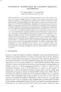
FIG. 1: Illustration of a critical region with corresponding errors of the first and second kind.
n2 during time t2 is obtained by simulating the experiment using only the established laws of physics. Since it is believed that the computer simulation correctly describes the data collection procedure, n2 can be regarded as drawn from the Poisson distribution with average background rate. In either case, a decision as to the plausibility of the existence of the phenomenon is made based on the outcomes of the two observations. Because the outcomes of the observations represent random numbers drawn from their respective parent distributions, the question of existence of the new phenomenon is here addressed by a hypothesis test. Various statistical tests have been developed which address the question of testing the hypothesis that two independent observations n1 and n2 made during times t1 and t2 are due to common background only. The methods, an overview of which can be found in [8], mostly use Gaussian-type approximations to the Poisson distribution and are not reliable for small numbers of observed events. In this paper we present the construction of the most powerful hypothesis test for this situation. That is, we calculate the critical region to be used which, for any given probability of claiming consistency with background fluctuation (typically a number such as 10−3 or less), maximizes the probability of detecting a signal. II.
TESTING A STATISTICAL HYPOTHESIS
We begin by reviewing the general procedure of hypotheses tests outlined in [4]. A statistical hypothesis is a statement concerning the distribution of a random variable Y .1 A hypothesis test is a rule for accepting or rejecting the hypothesis based on the outcome of an experiment. The hypothesis being tested, called the null hypothesis H0 , is formulated in such a way that all prior knowledge strongly supports it. The hypothesis is rejected if the 1
The variable Y may be a multidimensional vector. Throughout, we will use capital letters (such as Y ) to denote random variables and small letters (such as y) to denote their particular realizations.
3 observed value y of the random variable Y lies within a certain critical region w of the space W of all possible outcomes of Y and accepted or doubted otherwise. It follows, then, that if there are two tests for the same hypothesis H0 , the difference between them consists in the difference in critical regions. It also follows that H0 can be rejected when, in fact, it is true (error of the first kind ); or it can be accepted when some other alternative hypothesis H1 is true (error of the second kind ). The existence of an alternative hypothesis is clear, otherwise the null hypothesis would not be questioned. The probabilities of errors of these two kinds depend on the choice of the critical region. The definitions are illustrated in figure 1. Each probability p(y) of occurrence of every event y is given a subscript corresponding to its progenitor hypothesis, such as p0 (y) for H0 . The region to the right of yc is selected to be the critical one and the two types of errors of the test are marked with different hatching. A critical region is said to be the best critical region for testing hypothesis H0 with regard to H1 if it is the one which minimizes the probability of the error of the second kind (to accept H0 when H1 is true) among all regions which give the same fixed value of the probability of the error of the first kind (to reject H0 when it is true). The construction of the best critical region, resulting in the most powerful test of H0 with regard to H1 was considered in [4] where the problem is solved for the general case of simple hypotheses. A hypothesis is said to be simple if it completely specifies the probability of the outcome of the experiment; it is composite if the probability is given only up to some unspecified parameters. In general, if at least one of the hypotheses is composite, the best critical region may not exist [4]. Critical regions w(α) corresponding to different probabilities α of errors of the first kind are engineered before the test is performed. When experimental data y is obtained, the smallest α is found such that y ∈ w(α). It is then said, that the observed experimental data can be characterized by the p-value equal to α. The maximum p-value at which the null hypothesis is rejected is called significance of the test and will be denoted as αc . The corresponding critical region will be denoted as wc = w(αc ). The significance αc is set in advance, before the test is performed and its choice is based on the penalty for making the error of the first kind. (False scientific discoveries should not happen very often, and thus the significance is often selected as αc = 10−3 .) One minus the probability of the error of the second kind is called the power of the test which we denote as (1 − β). If as the result of the experiment the observed data lies inside of the critical region wc , it is concluded that the null hypothesis is rejected in favor of the alternative one with significance αc and power (1 − β). If, however, the observed data lies outside of the critical region wc , it is concluded that the null hypothesis is not rejected in favor of the alternative one with significance αc and power (1 − β). Special consideration must be given to the case of a composite null hypothesis H0 of the form p0 (y; {λ}) with unknown parameters {λ}. Indeed, suppose a critical region w is specified. Then, it is possible to perform the test: if the obtained value of the observable Y is inside the critical region w, the null hypothesis is rejected,Rif y 6∈ w, it is accepted. However, the probability of the error of the first kind α({λ}) = w p0 (y; {λ})dy in general depends on unknown values of parameters {λ} of the null hypothesis. Thus, the p-value α can not be assigned and the conclusion of the test can not be stated. It is therefore desired to construct such critical regions w, that the probability of the error of the first kind does not depend on the values of unknown parameters. Such regions are called similar to W with regard to parameters {λ}. A method for construction of such regions was found in [4] under limited conditions which in the case of one parameter λ are:
4 • the probability distribution p0 (y; λ) is infinitely differentiable with respect to λ and • the probability distribution p0 (y; λ) is such that if Φ(y) =
d log p0 , dλ
dΦ = A+B ·Φ dλ
then (1)
where the coefficients A and B are functions of λ, but are independent of observations y. If the above conditions are satisfied, critical regions w similar to W with regard to λ are built up of pieces of the hypersurfaces Φ = const defined by the likelihood ratio p1 /p0 > q. III.
NULL HYPOTHESIS BEING TESTED
As was pointed out above, in a typical counting-type experiment two independent observations yielding two counts n1 and n2 are made during time periods t1 and t2 respectively with all other conditions being equal. Because it is assumed that each event carries no information about another, each of the observed counts can be regarded as being drawn from a Poisson distribution with some value of the parameter. In as much as an attempt is being made to establish the existence of a new phenomenon, the null hypothesis H0 is formulated as: n1 and n2 constitute an independent sample of size 2 from a single Poisson distribution (adjusted for the duration of observation) which is due to a common background with some unknown count rate λ, or H0 :
p0 (n1 , n2 ) =
(λt1 )n1 (λt2 )n2 −λ(t1 +t2 ) e n1 ! n2 !
The alternative hypothesis is that the two observations are due to Poisson distributions with different unknown count rates λ1 and λ2 respectively (λ1 6= λ2 ): H1 :
p1 (n1 , n2 ) =
(λ1 t1 )n1 −λ1 t1 (λ2 t2 )n2 −λ2 t2 e e n1 ! n2 !
The usual physical situation is that one of the count rates is considered to have some amount due to the new process and the remainder due to the background process [e.g. λ1 = (λ + λsignal ) and λ2 = λ], thus the formulated hypothesis test matches the physical problem given in the introduction. It is seen that for the case of interest both hypotheses are of composite type (λ’s are unspecified) which complicates the construction of the test. IV.
THE MOST POWERFUL TEST
The formulated probability distribution p0 (n1 , n2 ) satisfies the conditions of a special case considered in [4], which facilitates the search for the best critical region in (n1 , n2 ) space. The probability distribution p0 (n1 , n2 ) satisfies the following conditions: • p0 (n1 , n2 ) is infinitely differentiable with respect to λ,
5 p0 • the function Φ(n1 , n2 ) defined as Φ(n1 , n2 ) = d log satisfies equation (1) with dλ n1 +n2 t1 +t2 1 Φ(n1 , n2 ) = λ − (t1 + t2 ), A = − λ and B = − λ .
Therefore, the best critical region corresponding to the error of the first kind α, determined from Φ = const, is built up of pieces of the lines nt = n1 + n2 = const. The segments of each line are those for which the ratio of likelihoods p1 /p0 is greater than some constant qα . This translates to: λ1 λ
! n1
λ2 λ
!nt −n1
e−(λ1 −λ)t1 e−(λ2 −λ)t2 ≥ qα
⇒
n1 ln
λ1 ≥ qα′ λ2
which can be written as: n1 ≥ nα , λ1 > λ2
(2)
n1 ≤ nα , λ1 < λ2
(3)
where the critical value nα is chosen to satisfy the desired probability of the error of the first kind α: α
nt X
p0 (k, nt − k) =
k=0
α
nt X
nt X
p0 (k, nt − k), λ1 > λ2
k=nα
p0 (k, nt − k) =
k=0
nα X
p0 (k, nt − k), λ1 < λ2
k=0
Substituting explicitly the expression for p0 (n1 , n2 ) in to these equations, we obtain α = (1 + γ)−nt
nt X
γ (n , n − n + 1), Cnkt γ k = I 1+γ α t α
λ 1 > λ2
(4)
λ 1 < λ2
(5)
k=nα
α = (1 + γ)−nt
nα X
k=0
Cnkt γ k = I
1 1+γ
(nt − nα , nα + 1),
n! where γ = t1 /t2 > 0, Cnm = m!(n−m)! are binomial coefficients and Ix (a, b) is the normalized incomplete beta function. It must be emphasized that the critical value nα depends on the parameters λ1,2 of the alternative hypothesis only via the relation λ1 < λ2 or λ1 > λ2 . The best critical region for testing the null hypothesis against the alternative with λ1 6= λ2 does not exist, but it does exist for testing against λ1 > λ2 or λ1 < λ2 separately, that is when the signal is a source or a sink respectively. The equations (4) with (2) or (5) with (3) define the best critical region w(α) in the space (n1 , n2 ) for testing H0 with regard to H1 (defined for λ1 < λ2 and λ1 > λ2 separately) corresponding to the probability of the error of the fist kind α. The boundary of this critical region is found by solving the equation (4) or (5) with respect to nα for all possible values of nt . Owing to the discrete nature of the observed number of events these equations might not have solutions for the specified level of significance αc . Nevertheless, it is possible to construct a conservative critical region such that the probability to observe data within the region does not exceed the preset level αc if the null hypothesis is true. This is done by requiring:
6
(
γ (n , n − n + 1) αc ≥ I 1+γ α t α γ (n − 1, n − n + 2) αc < I 1+γ α t α
αc
≥ I 1 (nt − nα , nα + 1) 1+γ αc < I 1 (nt − nα − 1, nα + 2)
λ 1 > λ2
λ 1 < λ2
1+γ
The power (1 − β) of the test will, of course, depend on the values of the parameters of the alternative hypothesis: (1 − β) =
nt ∞ X X
p1 (k, nt − k),
λ 1 > λ2
p1 (k, nt − k),
λ 1 < λ2
nt =0 k=nα
(1 − β) =
nα ∞ X X
nt =0 k=0
After explicit substitution of p1 (n1 , n2 ) into these equations, we obtain:
(1 − β) =
∞ X
λ 1 > λ2
(6)
∞ X
λ 1 < λ2
(7)
(λ1 t1 + λ2 t2 )nt −(λ1 t1 +λ2 t2 ) e I λ1 t1 (nα , nt − nα + 1), λ1 t1 +λ2 t2 nt ! nt =0
(λ1 t1 + λ2 t2 )nt −(λ1 t1 +λ2 t2 ) e I λ2 t2 (nt − nα , nα + 1), (1 − β) = λ1 t1 +λ2 t2 nt ! nt =0
For the purposes of the hypothesis test itself, equations (4,5) provide the method for the p-value calculation without the need for solving them. To do this, nt must be set to (n1 + n2 ) and nα to n1 then α is computed from the equation (4) or (5). If the obtained p-value α is not greater than αc the null hypothesis is rejected. This is the uniformly most powerful test of H0 with regard to H1 . It can be seen that the application of the method of best critical region construction [4] to the problem of testing whether two observations came from the Poisson distributions with the same parameter or not have led us to the criterion suggested on intuitive grounds in [6]. The presented discussion, however, shows that it is not possible to construct a better test for the hypotheses under consideration. The practical use of equations (4,5,6,7) should not present any difficulty using modern computers [5]. V.
COMPOUNDING RESULTS OF INDEPENDENT TESTS
It is often the case that the complete data set consists of several runs of the experiment, each of which belongs to the counting type subjected to Poisson distributed background with unknown means. The data set is then a set of pairs (n1,r , n2,r ) with corresponding durations of observations (t1,r , t2,r ), where subscript r enumerates all the runs of the experiment. Here we distinguish two cases: first where the parameters of both hypotheses do not depend on the run number r and second where such independence can not be asserted because of
7 modifications made to the apparatus between the runs. In the first case it can be seen that P the critical region must be constructed out of pieces of surfaces nt = r (n1,r + n2,r ) = const, P P on which r n1,r ≥ nα for the case of λ1 > λ2 or r n1,r ≤ nα for the case of λ1 < λ2 . It is thus seen that equations (4,5) provide a method for the p-value calculation: nt = P t1,r
+ n2,r ), nα = r n1,r and γ = Pr t2,r . In other words, if the parameters of both r hypotheses do not depend on the run number r, the corresponding observations can simply be added. In the second case, the derivation proceeds in the fashion similar to the presented derivation of equations (4,5), the critical region is built up of surfaces nt,r = n1,r + n2,r = const such that P
r (n1,r
P
X
n1,r log(λ1,r /λ2,r ) ≥ qα′
r
The critical value kind α:
qα′
α=
is chosen to satisfy the desired probability of the error of the first (1 + γr )−nt,r
Y r
(
X
r Cnkt,r γrkr
k ∈ [0, nt,r ] Pr ′ r kr log(λ1,r /λ2,r ) ≥ qα
The p-value is obtained by setting qα′ equal to r n1,r log(λ1,r /λ2,r ). In this case, the critical region depends on the parameters of the alternative hypothesis, but the test becomes uniformly most powerful if it is known that the ratios λ1,r /λ2,r do not depend on the run number r. The latter situation is common in practice because it reflects change of the level of pre-scaling of events in the data acquisition system or degradation of efficiency of sensors occurred between the experimental runs. P
VI.
CONCLUSION
In this paper we have reviewed the basic concepts of statistical hypothesis tests and underlined the relevant aspects often employed. The difficulty arises because frequently both the null and the alternative hypotheses are of composite type. We have considered typical counting experiments and constructed the most powerful statistical test. In doing so, we have insisted on the ability to quantify the error of the first kind although the parameter of the composite null hypothesis is unknown. The test also happens to be the uniformly most powerful with regard to the composite alternative hypothesis with λ1 < λ2 or λ1 > λ2 separately. The constructed test is especially important for the case of small number of events where previously used methods are inadequate because the usual Gaussian-type approximations break down. Fortuitously, this is the case for which the proposed test can most easily be performed. The existence of the most powerful statistical test allows comparisons with other computationally less demanding methods to be made which may be important for some applications. Acknowledgments
We would like to thank Prof. James Linnemann for helpful discussions and for making us aware of some relevant references.
8 This work is supported by the National Science Foundation (Grant Numbers PHY9901496 and PHY-0206656), the U. S. Department of Energy Office of High Energy Physics, the Los Alamos National Laboratory LDRD program and the Los Alamos National Laboratory Institute of Nuclear and Particle Astrophysics and Cosmology of the University of California.
[1] [2] [3] [4] [5]
D. Acosta et al. Phys. Rev. D, 65:111101(R), 2002. J. Ahrens et al. Phys. Rev. D, 66:032006, 2002. R. Atkins et al. Astrophys. J. Lett., 533:L119–L122, 2000. J. Neyman and E. S. Pearson. Philos. Trans. R. Soc. London, Series A, 231:289–337, 1933. W. H. Press, S. A. Teukolsky, W. T.Vetterling, and B. P. Flannery. Numerical Recipes in C: The Art of Scientific Computing. Cambridge University Press, second edition, 2002. [6] J. Przyborowski and H. Wilenski. Biometrika, 31:313–323, 1940. [7] E. M. Schlegel and R. Petre. Astrophys. J. Lett., 412:L29–L32, 1993. [8] S. N. Zhang and D. Ramsden. Experimental Astronomy, 1:145–163, 1990.