Hindawi Mathematical Problems in Engineering Volume 2018, Article ID 4368045, 14 pages https://doi.org/10.1155/2018/4368045
Research Article The Use of a Machine Learning Method to Predict the Real-Time Link Travel Time of Open-Pit Trucks Xiaoyu Sun,1 Hang Zhang ,1 Fengliang Tian,1 and Lei Yang2 1
Key Laboratory of Ministry of Education on Safe Mining of Deep Metal Mines, Northeastern University, Shenyang 110819, China School of Engineering, RMIT University, Melbourne, VIC 3000, Australia
2
Correspondence should be addressed to Hang Zhang;
[email protected] Received 16 January 2018; Revised 28 February 2018; Accepted 12 March 2018; Published 19 April 2018 Academic Editor: Panos Liatsis Copyright © 2018 Xiaoyu Sun et al. This is an open access article distributed under the Creative Commons Attribution License, which permits unrestricted use, distribution, and reproduction in any medium, provided the original work is properly cited. Accurate truck travel time prediction (TTP) is one of the critical factors in the dynamic optimal dispatch of open-pit mines. This study divides the roads of open-pit mines into two types: fixed and temporary link roads. The experiment uses data obtained from Fushun West Open-pit Mine (FWOM) to train three types of machine learning (ML) prediction models based on 𝑘-nearest neighbors (kNN), support vector machine (SVM), and random forest (RF) algorithms for each link road. The results show that the TTP models based on SVM and RF are better than that based on kNN. The prediction accuracy calculated in this study is approximately 15.79% higher than that calculated by traditional methods. Meteorological features added to the TTP model improved the prediction accuracy by 5.13%. Moreover, this study uses the link rather than the route as the minimum TTP unit, and the former shows an increase in prediction accuracy of 11.82%.
1. Introduction At present, shovel-truck systems (STSs) are commonly used in open-pit mining operations [1–3], especially for large open-pit mines. This is because STSs do not require extensive infrastructure in conjunction with a high mining intensity [4]. Although the trucks are very flexible, with a strong climbing ability, they also consume a large amount of fuel [5]. Related statistics showed that STSs contribute 50% of the operating costs in open-pit mines [6]. Therefore, almost all large open-pit mines are trying to optimize truck dispatching to achieve lower costs and higher mining efficiency [7–10]. Many open-pit mines have begun to use an open-pit automated truck dispatching system (OPATDS) in recent decades [9, 11]. Mining efficiency has increased through the integration of some truck dynamic dispatching principles (TDDPs) into the OPATDS [9, 11, 12]. The TDDPs rely heavily on an accurate truck cycle time [7, 8, 10], and one of its fundamental techniques is predicting the travel time of the trucks [11–14]. Several researchers have been working on travel time prediction (TTP) for open-pit trucks (OPTs) for many years.
Sun [15] first defined the average value for the predicted travel time of a truck based on artificial statistical data. However, the travel time is influenced by many factors, including truck type, load status, road properties, and weather conditions, making it difficult to predict the average travel time accurately and efficiently. Run-cai [16] used an artificial neural network (ANN) to predict the travel time of OPTs. Considering the randomness of TTP, they took several factors, namely, road conditions, truck type, and truck load status, into consideration. A total of 336 data records were used in their ANN model, and the results were better than those obtained using manual statistical methods. Jiangang [17] proposed a real-time dynamic TTP model based on the adaptive network-based fuzzy inference system (ANFIS) and discussed the theory and method of the ANFIS network. The ANFIS is a hybrid learning algorithm consisting of an error backpropagation algorithm, which performs with a higher calculation speed and better accuracy than the ANNs used in [16]. Chanda and Gardiner [18] compared the predictive capability of three truck cycle time estimation methods, that is,
2
Mathematical Problems in Engineering Table 1: Summary of the current state of TTP for OPTs.
Year 1998 2005 2005 2010 2010 2013 2013 2014
Authors Sun Run-cai Jiangang Chanda and Gardiner Xue et al. Edwards and Griffiths Erarslan Meng
Methods Manual statistics ANNs ANFIS ANNs, MRs, and TALPAC LS-SVR MRs and ANNs A computer-aided system BP-ANNs and SVM
computer simulation, ANN, and multiple regression (MR), in open-pit mining using TALPAC software and MATLAB. The results indicated that both the ANN and MR models showed better predictive abilities than the TALPAC model, which usually overestimated the travel time of longer haul routes while underestimating that of shorter haul routes. However, the difference between the time predicted by these two methods and the realistic travel time was insignificant. Edwards and Griffiths [19] attempted to predict the travel time of open-pit excavators through the development of ESTIVATE. Initially, ESTIVATE utilized a MR equation to predict the time, although it failed to provide an adequately robust predictor. Subsequently, improvement to ESTIVATE’s predictive capacity was sought through the use of ANNs, which provided a significant improvement over the MR approach. Erarslan [20] focused on the truck speed and developed a computer-aided system to estimate the speed data for different resistances. Then, the truck travel time was equivalent to the length of the road divided by the truck speed. Considering the various influencing factors on TTP, Xue et al. [21] proposed a dynamic prediction method that comprised an ensemble learning algorithm using least squares support vector regression (LS-SVR). The results obtained from the MATLAB model showed the effectiveness and high accuracy of their algorithms. Meng [22] compared the support vector machine (SVM) approach with the backpropagation (BP) algorithm and observed that the SVM model performed with a higher accuracy than the BP neural network model in TTP. Reported studies on the TTP of OPTs are summarized in Table 1. Several aspects of the table require further discussion: (1) Most of the existing studies have considered openpit roads as a single category. Unlike urban traffic networks, there are many temporary roads in openpit mines, for example, coal mines in Kuzbass, where temporary roads constitute up to 80% of the total road length [23]. A TTP model based on commonly fixed roads may not be reliable because the temporary roads between load and dump points change frequently. (2) Most experiments reported in the literature were based on the route travel time prediction (RTTP), although the number of routes from A to B exceeds
Conclusions An available method Better than [15] Better than [16] Each has its advantages An available method ANN is better than MR An available method SVM is better than BP-ANN
Ref. [15] [16] [17] [18] [21] [19] [20] [22]
one. Thus, the RTTP with uncertainty must be improved. (3) Reported studies have seldom considered the meteorological factors when the open-pit mine is extracting. For example, snow or heavy rain decreases the speed of trucks and has an adverse effect on the travel time of vehicles [24–27]. (4) Available predictive models have been based on small-scale datasets; for example, only hundreds of data records were used in [15–17, 21]. Better results are usually obtained when using large-scale training datasets. With the rapid development of machine learning (ML) and big data technology, the TTP of OPTs is expected to become faster and more accurate. In this study, the primary objectives and improved measures are as follows: (1) The open-pit mine roads are divided into two types: long-term fixed roads and temporary roads. Experiments explore the results of TTP on the two different types of roads. (2) This paper uses the link rather than the route as the minimum prediction unit. The difference between the link and route is that the route contains multiple road nodes. Independent TTP models are used to train each link road instead of using the same TTP model for the entire road network. (3) The experiments in this paper explore the impact of meteorological conditions on TTP, which means meteorological features are added to the model training process. (4) The OPATDS database stores a large amount of truck condition data. For large-scale data, machine learning methods tend to have good prediction performance. More than a million records are used to train the link travel time prediction (LTTP) model in this study.
2. Models and Experiments 2.1. Experimental Roadmap and Methods. As shown in Figure 1, Fushun West Open-pit Mine (FWOM, Fushun Mining Group Co., Ltd.) is located in Fushun city, Liaoning province,
Mathematical Problems in Engineering
3
Fushun
Fushun Beijing
Shanghai 300 km
Fushun West Open-pit Mine
Figure 1: Location of the Fushun West Open-pit Mine.
1200
Dump A
Load D
Node B
Y-axis of FWOM
1000 Node E
Load C Load F
800
Load G 600 Node J
400 300
Node H 500
1000
1500 2000 X-axis of FWOM
2500
3000
Fixed roads Temporary roads
Figure 2: Experimental roadmap of the FWOM.
China, approximately 50 km east of Shenyang. The FWOM is the largest open-pit coal mine in Asia and produces an estimated 1.5 billion tons of coal [28]. The roadmap used in this experiment is shown in Figure 2, which is part of the road networks of the FWOM. The nodes of transportation roads typically remain the same at a specified time, whereas roads to load points and dump points change with mining activities. According to the changing road nodes, link roads can be divided into two categories: (1) Fixed link roads, for example, the link roads between node B and node E, node E and node H, and node H and node J. (2) Temporary link roads, for example, the link roads between node B and node D, node E and node F, and node G and node H. ML, which is a field of computer science, gives computers the ability to learn without being explicitly programmed [35, 36]. ML is related to computational statistics and suitable
for predicting tasks because of its self-adaptation and selffeedback characteristics [37, 38]. An experimental flow chart used in the ML method is given in Figure 3. Note that the LTTP model of each experimental link road is independently trained. Figure 3 shows the three steps of LTTP using ML. As the most crucial step, training the LTTP model consists of two parts: ML algorithms and training data. These two parts are indispensable because training the ML prediction models requires a large amount of data provided by the OPATDS. In the second step, LTTP model predictions are obtained from the test data, and the prediction performance of the model can also be evaluated. The final step involves modifying the parameters of the LTTP model until the result is acceptable. In particular, the test dataset is a dataset that is independent of the training dataset [39]. 2.2. ML Algorithms Selection. ML tasks are typically classified into four broad categories [40]: supervised learning, unsupervised learning, reinforcement learning, and semisupervised
4
Mathematical Problems in Engineering LTTP model 2 Test data
Machine learning algorithm
1 3 Results & evaluation
Training data
Figure 3: Experimental flowchart of ML methods.
Table 2: Adaptability analysis between ML algorithms and LTTP. Algorithms ANNs BNs SVM RF LR kNN DT HM
Adaptability analysis The effect has been thoroughly verified by many existing studies. A probabilistic model that is not suitable for this study [29]. Perfect theoretical basis with high generalization ability [30]. An ensemble learning method evolved from DT; better than DT [31]. It solves the classification problems; not suitable for this study [32]. An efficient algorithm for the classification and regression tasks [33]. RF has been chosen; there is no need to choose DT. A probabilistic model that is not suitable for this study [34].
learning [41]. The LTTP of OPTs belongs to the typical supervised learning task due to the labeled training data from the OPATDS [42]. Prediction models output the travel time values of OPTs, which can be considered to be a regression problem of supervised learning. There are many ML algorithms that can be used to solve the regression problem of supervised learning, such as ANN, Bayesian network (BN), SVM, random forest (RF), logistic regression (LR), 𝑘-nearest neighbors (kNN), decision tree (DT), AdaBoost [43], and hidden Markov model (HM) approaches [44]. The adaptability analysis between LTTP and the various ML algorithms is given in Table 2. Based on the comparison results, this paper chooses the kNN, SVM, and RF algorithms to build the LTTP models of OPTs. kNN is a nonparametric method used for classification and regression, and the kNN regression computes the mean of the function values of its 𝑘-nearest neighbors [33, 45]. The goal function regression 𝑓kNN (𝑥) of kNN regression is written as follows [45]: 𝑓kNN (𝑥) =
1 ⋅ ∑ 𝑦, 𝑘 𝑖∈𝑁 (𝑥) 𝑖
(1)
𝑘
where 𝑥 is an unknown pattern; 𝑁𝑘 (𝑥) is the indices of the 𝑘-nearest neighbors of 𝑥; and 𝑦𝑖 is the predicted labels. The original SVM algorithm was invented by Cortes and Vapnik [46], and its efficiency in classification has been verified in many case studies [47]. The detailed introduction of SVM can be found in Smola and Sch¨olkopf [48], in which they published the complete tutorial on support vector
Apply No No Yes Yes No Yes No No
regression. To train the SVM regression model, the following must be solved: 1 (2a) minimize ‖𝑤‖2 2 subject to 𝑦𝑖 − ⟨𝑤, 𝑥𝑖 ⟩ − 𝑏 ≤ 𝜀 ⟨𝑤, 𝑥𝑖 ⟩ + 𝑏 − 𝑦𝑖 ≤ 𝜀,
(2b)
where 𝑥𝑖 represents the training features with target value 𝑦𝑖 ; ⟨𝑤, 𝑥𝑖 ⟩ + 𝑏 is the prediction value; and 𝜀 is a free parameter that serves as a threshold. The RF algorithm evolved from DT theory and was created by Ho in 1995 [31]. This approach incorporates the bootstrap aggregating (Bagging) algorithm, which is a method for generating multiple versions of a predictor and then using these to obtain an aggregated predictor [49]. The RF method has a higher degree of efficiency and accuracy than the DT method because of Bagging. 2.3. Training Data Structure. The training dataset is the most critical factor when training ML prediction models, and it consists of several features and corresponding target values [50]. Many features commonly affect the LTTP of OPTs, which can be broadly classified into three categories: truck features, road features, and meteorological features. The meteorological features are considered in this paper because rainy and snowy weather reduces both the friction coefficient of roads and the truck driver’s vision. According to the relevant statistics reported by the U.S. Federal Highway Administration, bad weather can lead to a 35% reduction in car speed [51].
Mathematical Problems in Engineering
5
Table 3: Preprocessed data for training the ML prediction models. Date
Start time
Arrival time
Truck Id
Truck type
2017-03-01 2017-03-02
16:23:20 20:12:09
16:26:57 20:18:12
202 503
BELAZ-L MT-86
Truck status
𝑥-axis start
𝑦-axis start
𝑥-axis arrival
𝑦-axis arrival
1344 2576
1188 783
Load status
Start node
Arrival node
2191 3095 Pressure (100 Pa)
968 327 Wind speed (m/s)
Empty Coal Temperature (∘ C)
B G Relative humidity (%)
E H Precipitation (mm)
1002 999
1 0.6 Travel time (hour:min:sec)
90 96
0 0
Run Run
2 1
Rain No No
00:03:37 00:06:03
Table 4: Description of the variables used in the prediction. Variables Truck Id Truck type Truck status 𝑥-axis start 𝑦-axis start 𝑥-axis arrival 𝑦-axis arrival Load status Start node Arrival node Pressure Wind speed Temperature Relative humidity Precipitation Rain Travel time
Type
Role
Description
Numeric Categorical Categorical Numeric Numeric Numeric Numeric Categorical Categorical Categorical Numeric Numeric Numeric Numeric Numeric Categorical Date time
Feature Feature Feature Feature Feature Feature Feature Feature Feature Feature Feature Feature Feature Feature Feature Feature Target
The serial number of truck. The type of the truck (i.e., BELAZ-L, BELAZ-M, and MT86). The status of the truck (i.e., running, waiting, and stop). The 𝑥 coordinate of the truck at the starting position. The 𝑦 coordinate of the truck at the starting position. The 𝑥 coordinate of the truck at the ending position. The 𝑦 coordinate of the truck at the ending position. The load status of the truck (i.e., empty and coal). The node code of the starting position of the road. The node code of the ending position of the road. A fundamental atmospheric quantity. A fundamental atmospheric quantity. A fundamental atmospheric quantity. A fundamental atmospheric quantity. A fundamental atmospheric quantity. A fundamental atmospheric quantity (i.e., yes and no). The travel time of the truck on each link.
The data used in the following experiments originate from the FWOM. The truck and road feature data are from the OPATDS, while the weather data are collected from the China Meteorological Administration (CMA) Number 54351 monitoring station. The preprocessed training dataset samples in this experiment are listed in Table 3. There are 16 variables serving as the features, and the target is the truck travel time. Table 4 shows the description of the target and each feature used for the prediction in this study. 2.4. Program and Pseudocode. This study used sophisticated algorithms to predict the link travel time in open-pit mines, and the three ML algorithms in the prediction models were based on scikit-learn, which is an open-source ML module in
the Python programming language [52, 53]. The pseudocode of the methodology in this study is illustrated in Figure 4.
3. Results and Discussion 3.1. Predictions of the ML Models. For the training datasets, 2,246,746 historical records from March 2017 were exported from the OPATDS database of the FWOM. After data preprocessing, the structure of the training data was similar to those in Table 3. The experimental parameters encompassed one type of link road trained by three different ML algorithms (kNN, SVM, and RF) resulting in 18 LTTP models. The prediction results for the last 50 records of the test datasets are shown in Figure 5.
6
Mathematical Problems in Engineering
Figure 4: The pseudocode of the ML methodology.
To derive the best LTTP model for each link road, the aforementioned prediction results were evaluated based on the mean absolute deviation (MAD) and the mean absolute percentage error (MAPE) methods, which are commonly used for regression problem evaluation. The MAD, as expressed in (3a), is a summary statistic of statistical dispersion or variability [54, 55]. The MAPE is a measure of the accuracy of a prediction method in statistics, as written in (3b) [56]. Because the MAPE is a percentage, it is often easier to understand than the other statistics. For example, if the MAPE is 5, on average, the forecast is off by 5% [57]. MAD =
∑𝑛𝑖=1 𝑥obs,𝑖 − 𝑥model,𝑖 , 𝑛
∑𝑛 (𝑥obs,𝑖 − 𝑥model,𝑖 ) /𝑥obs,𝑖 × 100 (%) , MAPE = 𝑖=1 𝑛
(3a)
where 𝑥obs,𝑖 represents the observation values; 𝑥model,𝑖 represents the prediction values; and 𝑛 is the number of data records. Table 5 lists the MAD and MAPE values obtained from the three ML methods for each experimental link road. Smaller MAD and MAPE values reflect better prediction performance of each LTTP model, and the smallest records are highlighted in Table 5. The results of the six experimental link roads indicate that the LTTP models built using the SVM and RF methods are better than those using the kNN algorithm. Table 6 summarizes the optimal ML prediction models for each link road. The coefficient of determination, 𝑅2 , is widely used in statistical tests to evaluate the predictive capability of a model and is also used in this study. The 𝑅2 value with one independent variable is written as follows [58]: 2
(3b)
𝑅2 = [
(𝑥 − 𝑥) ∗ (𝑦𝑖 − 𝑦) 1 ] , ∗∑ 𝑖 𝑁 (𝜎𝑥 ∗ 𝜎𝑦 )
(4)
00:09:00 00:08:00 00:07:00 00:06:00 00:05:00 00:04:00 00:03:00 0
5
10
15
20
25 30 B-D
35
40
45
00:02:00
50
00:12:00
00:10:00
00:11:00
00:09:00
00:10:00
00:08:00
00:09:00
Link travel time
00:11:00
00:07:00 00:06:00 00:05:00 00:04:00
00:12:00 00:11:00 00:10:00 00:09:00 00:08:00 00:07:00 00:06:00 00:05:00 00:04:00 00:03:00 00:02:00 00:01:00
15
20
25 30 E-F
35
40
45
00:02:00
50
15
20
25 30 B-E
35
40
45
50
0
5
10
15
20
25 30 E-H
35
40
45
50
0
5
10
15
20
25 30 H-J
35
40
45
50
00:05:00 00:03:00
10
10
00:06:00 00:04:00
5
5
00:07:00
00:02:00 0
0
00:08:00
00:03:00 00:01:00
Link travel time
00:10:00
Link travel time
00:22:00 00:21:00 00:20:00 00:19:00 00:18:00 00:17:00 00:16:00 00:15:00 00:14:00 00:13:00 00:12:00 00:11:00 00:10:00 00:09:00 00:08:00 00:07:00 00:06:00 00:05:00 00:04:00
7
00:08:00 00:07:00 Link travel time
Link travel time
Link travel time
Mathematical Problems in Engineering
00:06:00 00:05:00 00:04:00 00:03:00 00:02:00
0
5
10
15
Raw value KNN
20
25 30 G-H
35
40
45
50
SVM RF
00:01:00
Raw value KNN
SVM RF
Figure 5: Prediction results for the different ML methods.
where 𝑁 is the number of observations used to fit the model; 𝑥 and 𝑦 are the mean values of 𝑥 and 𝑦, respectively; 𝑥𝑖 and 𝑦𝑖 are the values of observation 𝑖; and 𝜎𝑥 and 𝜎𝑦 are the standard deviations of 𝑥 and 𝑦, respectively. Table 7 shows the 𝑅2 values of the three ML models for each link road. The 𝑅2 values range from 0 to 1, and 𝑅2 equal to 1 indicates perfect accurate prediction. There are some differences between Tables 6 and 7, that is, the optimal ML model of B-E, H-J, and G-H. However, the MAPE was still selected for choosing the optimal model because the 𝑅2 value cannot be used to evaluate predictive errors.
3.2. Discussion of Traditional Averaging Methods and ML Models. To compare the LTTP of ML models and traditional averaging methods, controlled experiments were performed. The flow chart of traditional averaging methods is illustrated in Figure 6. For each record in the test dataset, the experiments traced back the corresponding top 10, 20, 30, 40, and 50 records and then calculated the average value as the final prediction. To improve the accuracy of the traditional averaging methods, each calculation used only historical data for the same truck type and load status. The results obtained
8
Mathematical Problems in Engineering Table 5: LTTP evaluation based on the different ML models.
Link road
Road type
Evaluation MAD MAPE MAD MAPE MAD MAPE MAD MAPE MAD MAPE MAD MAPE
B-E E-H
Fixed
H-J B-D E-F
Temporary
G-H
1
Data predicted
kNN 5.91𝐸 − 04 1.78𝐸 + 01 9.44𝐸 − 04 2.49𝐸 + 01 5.16𝐸 − 04 2.14𝐸 + 01 1.71𝐸 − 03 2.75𝐸 + 01 9.59𝐸 − 04 3.13𝐸 + 01 1.18𝐸 − 03 3.42𝐸 + 01
SVM 5.09𝐸 − 04 1.58𝐸 + 01 3.32E − 04 9.57E + 00 3.55𝐸 − 04 1.59𝐸 + 01 5.44E − 04 8.09E + 00 8.05𝐸 − 04 2.94𝐸 + 01 7.35E − 04 1.94E + 01
B-E
BELAZ
Empty
??:??:??
B-E
BELAZ
Empty
00:13:57
B-E
MT-86
Empty
00:17:15
00:13:57
B-E
MT-86
Load
00:18:21
00:14:21
B-E
BELAZ
Empty
00:14:21
RF 4.56E − 04 1.44E + 01 6.37𝐸 − 04 1.81𝐸 + 01 3.54E − 04 1.48E + 01 6.70𝐸 − 04 9.90𝐸 + 00 5.63E − 04 1.82E + 01 7.85𝐸 − 04 2.38𝐸 + 01
00:14:09
2
Recent historical data
4
3 Calculating the average time: (i) Same link road (ii) Same load status (iii) Same truck type
Figure 6: The flow chart of traditional averaging methods.
Table 6: Summary of the optimal ML prediction models for each link road. Road B-E E-H H-J B-D E-F G-H
Type
Optimal ML model RF SVM RF SVM RF SVM
Fixed
Temporary
smallest records are highlighted in Table 8. The predicted values obtained from the optimal ML method and a traditional average method for each link road are given in Table 9; the decrease in the MAPE is also shown. Table 9 shows that the tested ML models are superior to the traditional averaging method in the context of LTTP because the former has smaller MAPEs. An average increase of 15.79% in prediction accuracy is achieved in all experimental link roads, in which increases of 12.54% and 19.30% for three fixed and three temporary roads, respectively, are also obtained.
Table 7: 𝑅2 values of the different ML models for each link road. Road B-E E-H H-J B-D E-F G-H
SVM 0.28 0.83 0.72 0.89 0.54 0.61
KNN 0.16 0.16 0.13 0.23 0.24 0.19
RF 0.41 0.67 0.56 0.7 0.73 0.62
Optimal ML model SVM SVM SVM SVM RF RF
from the traditional averaging methods are summarized in Table 8. Smaller MAD and MAPE values mean better prediction performance of the traditional averaging methods, and the
3.3. Discussion of Meteorological Features. This study also considered the influence of meteorological features on the LTTP of an open-pit mine. The data were obtained from a CMA monitoring station, including 5 variables: pressure, wind speed, temperature, relative humidity, and precipitation. The Pearson correlation coefficient (PCC), an evaluation method developed by Pearson [59], was used to evaluate the linear correlation between two variables. The expression of the PPC is as follows: 𝜌𝑋,𝑌 =
cov (𝑋, 𝑌) , 𝜎𝑋 𝜎𝑌
(5)
Mathematical Problems in Engineering
9
Table 8: Results obtained from the traditional averaging methods. Road B-E E-H H-J B-D E-F G-H
Evaluation
10 records 1.02𝐸 − 03 3.06𝐸 + 01 1.22𝐸 − 03 3.29𝐸 + 01 6.29𝐸 − 04 2.54𝐸 + 01 2.15𝐸 − 03 3.17𝐸 + 01 1.16𝐸 − 03 3.91𝐸 + 01 1.29E − 03 4.04E + 01
MAD MAPE MAD MAPE MAD MAPE MAD MAPE MAD MAPE MAD MAPE
20 records 9.49𝐸 − 04 2.81𝐸 + 01 1.13𝐸 − 03 3.00𝐸 + 01 6.09𝐸 − 04 2.47𝐸 + 01 1.83E − 03 2.69E + 01 1.10E − 03 3.63E + 01 1.38𝐸 − 03 4.12𝐸 + 01
Traditional averaging methods 30 records 9.17𝐸 − 04 2.66𝐸 + 01 1.09𝐸 − 03 2.84𝐸 + 01 5.87𝐸 − 04 2.36𝐸 + 01 2.46𝐸 − 03 3.86𝐸 + 01 1.14𝐸 − 03 3.81𝐸 + 01 1.36𝐸 − 03 3.91𝐸 + 01
40 records 9.18𝐸 − 04 2.64𝐸 + 01 1.09𝐸 − 03 2.81𝐸 + 01 5.81𝐸 − 04 2.34𝐸 + 01 2.36𝐸 − 03 3.62𝐸 + 01 1.15𝐸 − 03 3.90𝐸 + 01 1.32𝐸 − 03 3.70𝐸 + 01
50 records 9.04E − 04 2.58E + 01 1.07E − 03 2.73E + 01 5.80E − 04 2.33E + 01 2.05𝐸 − 03 3.25𝐸 + 01 1.16𝐸 − 03 3.95𝐸 + 01 1.30𝐸 − 03 3.57𝐸 + 01
Table 9: Comparison between the optimal ML model and the optimal averaging method. Road B-E E-H H-J B-D E-F G-H Average
Type Fixed
Temporary
Optimal average method (MAPE) 2.58𝐸 + 01 2.73𝐸 + 01 2.33𝐸 + 01 2.69𝐸 + 01 3.63𝐸 + 01 4.04𝐸 + 01
Optimal ML model (MAPE) 1.44𝐸 + 01 9.57𝐸 + 00 1.48𝐸 + 01 8.09𝐸 + 00 1.82𝐸 + 01 1.94𝐸 + 01
MAPE decrease 11.40% 17.73% 8.50% 18.81% 18.10% 21.00%
Average 12.54%
19.30% 15.79%
Table 10: Prediction results after including meteorological data. Type
Temporary
Fixed
Road
Methods
B-E
RF
E-H
SVM
H-J
RF
B-D
SVM
E-F
RF
G-H
SVM
Meteorological features No Yes No Yes No Yes No Yes No Yes No Yes
Average
where cov(𝑋, 𝑌) is the covariance; 𝜎𝑋 is the standard deviation of 𝑋; and 𝜎𝑌 is the standard deviation of 𝑌. The PPC values of different variables are shown in Figure 7, including the 5 meteorological variables and truck travel time. A high PCC value indicates a closer relationship between the two variables. Following controlled experiments, the effect of meteorological features was investigated by adding or removing individual features. We selected the optimal ML model for
MAD 6.90𝐸 − 04 4.56𝐸 − 04 3.41𝐸 − 04 3.32𝐸 − 04 4.16𝐸 − 04 3.54𝐸 − 04 6.35𝐸 − 04 5.44𝐸 − 04 6.60𝐸 − 04 5.63𝐸 − 04 8.42𝐸 − 04 7.35𝐸 − 04
MAPE 2.07𝐸 + 01 1.44𝐸 + 01 1.69𝐸 + 01 9.57𝐸 + 00 1.86𝐸 + 01 1.48𝐸 + 01 1.22𝐸 + 01 8.09𝐸 + 00 2.17𝐸 + 01 1.82𝐸 + 01 2.52𝐸 + 01 1.94𝐸 + 01
MAPE decrease (no-yes)% 6.30% 7.28% 3.80% 4.08% 3.50% 5.80% 5.13%
each link road. The raw (observation) values and predicted results with/without meteorological features are shown in Figure 8. The results of the controlled experiments are shown in Table 10; the calculated decrease in the MAPE is also shown. The results considering meteorological features are better than those without meteorological features. The MAPE decreased by 5.13% on average for all link roads after adding the meteorological data.
10
Mathematical Problems in Engineering
1
−0.48
−0.48
Wind speed −0.48
1
0.47
Temperature −0.48
0.47
1
Pressure
0.64
−0.041 −0.019
−0.82 −0.088 −0.64
0.14
0.05
0.8
0.4
0.049 0.0
Precipitation −0.041 −0.088
0.12
0.12 −0.054 1
0.049 −0.054 0.045 Precipitation
0.05 Wind speed
Pressure
Travel time −0.019
0.14
1
0.045
−0.4
−0.8
1 Travel time
−0.82 −0.64
Relative humidity
0.64
Temperature
Relative humidity
Figure 7: The PCC heat map of meteorological features. Table 11: Evaluation of LTTP based on different ML models. Link road A-B
Road type Fixed
Evaluation MAD MAPE
3.4. Discussion of LTTP and RTTP. The above experiments used the link rather than the route to predict the travel time of OPTs. However, the differences between LTTP and RTTP need to be further discussed. In the ensuing discussion, the longest route between dump point A and load point G is selected, as shown in Figure 9. The A-G route consists of 4 links: A-B, B-E, E-H, and HG. Among them, the optimal ML prediction models of B-E, E-H, and H-G are SVM, RF, and SVM, respectively. The same experimental procedure as used in Section 3.1 was used to obtain the optimal ML model for A-B, and Table 11 shows the MAD and MAPE values of the three ML methods. It can be seen that the RF model is the best ML method for link A-B. The SVM and RF methods are used to predict the RTTP of A-G because those two models have a good prediction performance. Thus, the experiments are summarized as follows: (i) RTTP (SVM): using the SVM algorithm to train the TTP model for the route A-G. (ii) RTTP (RF): using the RF algorithm to train the TTP model for the route A-G. (iii) LTTP: using the optimal ML model for each link, that is, A-B (RF), B-E (SVM), E-H (RF), and H-G (SVM), and the truck travel time of A-G is the sum of each LTTP result. Raw values and predicted results of the above three experiments are shown in Figure 10, while the evaluated
kNN 4.95𝐸 − 04 4.69𝐸 + 01
SVM 3.28𝐸 − 04 3.40𝐸 + 01
RF 2.99E − 04 3.36E + 01
Table 12: Evaluation of the results between LTTP and RTTP. Method
Model
RTTP
SVM
RTTP
RF
LTTP
Assemble
Evaluation MAD MAPE MAD MAPE MAD MAPE
Values 1.55𝐸 − 03 2.08𝐸 + 01 1.78𝐸 − 03 2.35𝐸 + 01 8.34E − 04 8.98E + 00
results of those experiments are shown in Table 12. Both the MAD and MAPE values of the LTTP approach are smaller than the two RTTP methods. Thus, using the link as the prediction unit is better than using the route.
4. Conclusions The link roads of an open-pit mine are divided into fixed and temporary roads in this paper. Three ML algorithms, that is, kNN, SVM, and RF, are used for the LTTP of OPTs. The experimental results not only reflect the self-adaptive and self-feedback characteristics of the ML algorithms but also demonstrate the practicality of the method for road segments. The conclusions based on the results are as follows: (1) LTTP models based on ML are more efficient and accurate than traditional averaging methods. An overall average increase of 15.79% in the prediction accuracy is obtained for six experimental link roads.
00:22:00 00:21:00 00:20:00 00:19:00 00:18:00 00:17:00 00:16:00 00:15:00 00:14:00 00:13:00 00:12:00 00:11:00 00:10:00 00:09:00 00:08:00 00:07:00 00:06:00 00:05:00 00:04:00
11 00:10:00 00:09:00 00:08:00 Link travel time
Link travel time
Mathematical Problems in Engineering
0
5
10
15
20 25 30 B-D (SVM)
35
40
45
0
5
10
15
20 25 30 B-E (RF)
35
40
45
50
0
5
10
15
20 25 30 E-H (SVM)
35
40
45
50
0
5
10
15
20 25 30 H-J (RF)
35
40
45
50
00:11:00 00:10:00
00:06:00
Link travel time
Link travel time
00:04:00
00:12:00
00:05:00 00:04:00 00:03:00
00:09:00 00:08:00 00:07:00 00:06:00 00:05:00 00:04:00
00:02:00
00:03:00 0
5
10
15
20 25 30 E-F (RF)
35
40
45
00:02:00
50
00:08:00 00:07:00 Link travel time
Link travel time
00:05:00
00:02:00
50
00:07:00
00:12:00 00:11:00 00:10:00 00:09:00 00:08:00 00:07:00 00:06:00 00:05:00 00:04:00 00:03:00 00:02:00 00:01:00
00:06:00
00:03:00
00:08:00
00:01:00
00:07:00
00:06:00 00:05:00 00:04:00 00:03:00 00:02:00
0
5
10
15
20 25 30 G-H (SVM)
35
40
45
50
Raw value Without meteorological features Meteorological features
00:01:00
Raw value Without meteorological features Meteorological features
Figure 8: Comparison forecast results including and excluding meteorological features.
For temporary roads, the average accuracy increases by 19.30%.
that considering the effect of meteorological features on LTTP increases the prediction accuracy by 5.13%.
(2) LTTP models established using the SVM and RF algorithms are better than those established using the kNN approach. There is no large difference between the SVM and RF results, although the RF algorithm requires less space and time complexity than the SVM algorithm.
(4) The differences between LTTP and RTTP are also discussed, and the former has a higher prediction accuracy. The MAPE decreases by 11.82% for the LTTP method.
(3) This paper is original in that it considers the effect of meteorological features on LTTP. The results show
Some work is already underway to incorporate the ML prediction models into the OPATDS of the FWOM, which will be helpful in improving the dispatching efficiency of the OPTs.
12
Mathematical Problems in Engineering Dump A
Load D
Node B
Node E
Load C Load F
Load G
Node J Node H
!
Fixed roads Temporary roads
Truck travel time
Figure 9: The location of the route A-G in the FWOM roadmap.
00:22:00 00:20:00 00:18:00 00:16:00 00:14:00 00:12:00 00:10:00 00:08:00 00:06:00
References [1] J. Czaplicki, Shovel-Truck Systems, CRC Press, 2008. [2] J. M. Czaplicki, “Modelling and analysis of the exploitation process of a shovel-truck system,” in Shovel-Truck Systems, pp. 79–89, CRC Press, 2008.
0
5
10
15
20 25 30 35 Route A-G
40
45
50
[3] S. G. Ercelebi and A. Bascetin, “Optimization of shovel-truck system for surface mining,” Journal of the Southern African Institute of Mining and Metallurgy, vol. 109, no. 7, pp. 433–439, 2009.
Figure 10: Prediction results for RTTP (RF), RTTP (SVM), and LTTP.
[4] R. Mena, E. Zio, F. Kristjanpoller, and A. Arata, “Availabilitybased simulation and optimization modeling framework for open-pit mine truck allocation under dynamic constraints,” International Journal of Mining Science and Technology, vol. 23, no. 1, pp. 113–119, 2013.
Data Availability
[5] F. Soumis, J. Ethier, and J. Elbrond, “Truck dispatching in an open pit mine,” International Journal of Surface Mining, Reclamation and Environment, vol. 3, no. 2, pp. 115–119, 1989.
Raw values RTTP (RF)
RTTP (SVM) LTTP
The data used to support the findings of this study are available from the corresponding author upon request.
Conflicts of Interest
[6] A. Y. F. Fadin, Komarudin, and A. O. Moeis, “Simulationoptimization truck dispatch problem using look - ahead algorithm in open pit mines,” International Journal of GEOMATE, vol. 13, no. 36, pp. 80–86, 2017.
Authors’ Contributions
[7] Y. Tan and S. Takakuwa, “A practical simulation approach for an effective truck dispatching system of open pit mines using VBA,” in Proceedings of the 2016 Winter Simulation Conference, WSC 2016, pp. 2394–2405, IEEE, Washington, DC, USA, December 2016.
Xiaoyu Sun, as the principal investigator, provided the data used to train the ML models. Hang Zhang performed the experiments and wrote the paper. Fengliang Tian contributed the programming. Lei Yang proofread the manuscript.
[8] J. Li, R. Bai, J. Mao, and W. Li, “Forecast of applied effect for truck real-time dispatch system in open-pit mine based on CSUSS,” in Proceedings of the 2010 International Conference on E-Product E-Service and E-Entertainment, ICEEE2010, pp. 1–4, IEEE, Henan, China, November 2010.
Acknowledgments
[9] S. P. Alarie and M. Gamache, “Overview of solution strategies used in truck dispatching systems for open pit mines,” International Journal of Surface Mining, Reclamation and Environment, vol. 16, no. 1, pp. 59–76, 2002.
The authors declare no conflicts of interest.
This work was funded by the National Natural Science Foundation of China (no. 51674063) and the National Key Research and Development Program of China (no. 2016YFC0801608).
[10] B. Kolonja, D. R. Kalasky, and J. M. Mutmansky, “Optimization of dispatching criteria for open-pit truck haulage system design using multiple comparisons with the best and common random
Mathematical Problems in Engineering
[11]
[12]
[13]
[14]
[15] [16]
[17]
[18]
[19]
[20]
[21]
[22]
[23]
[24]
[25]
[26]
numbers,” in Proceedings of the 25th Conference on Winter Simulation, WSC 1993, pp. 393–401, ACM, Los Angeles, California, USA, December 1993. Q. Wang, Y. Zhang, C. Chen, and W. Xu, “Open-pit mine truck real-time dispatching principle under macroscopic control,” in Proceedings of the 1st International Conference on Innovative Computing, Information and Control 2006, ICICIC’06, pp. 702– 705, IEEE, Beijing, China, September 2006. Y. Choi, “Simulation of Shovel-Truck Haulage Systems by Considering Truck Dispatch Methods,” Journal of the Korean Society of Mineral and Energy Resources Engineers, vol. 50, no. 4, p. 543, 2013. E. Topal and S. Ramazan, “Mining truck scheduling with stochastic maintenance cost,” Journal of Coal Science and Engineering, vol. 18, no. 3, pp. 313–319, 2012. P. Chaowasakoo, H. Sepp¨al¨a, H. Koivo, and Q. Zhou, “Digitalization of mine operations: Scenarios to benefit in real-time truck dispatching,” International Journal of Mining Science and Technology, vol. 27, no. 2, pp. 229–236, 2017. Q. Sun, “Road running time statistics method in truck scheduling,” Opencast Coal Mining Technology, vol. 01, pp. 35–37, 1998. R. Bai, J. Li, and J. Xu, “Real-time dynamic forecast of truck link travel time,” Journal of Liaoning Technical University, vol. 1, pp. 12–14, 2005. L. Jiangang, “Real-time dynamic forecasts of truck link travel time based on fuzzy neural network,” Journal of the China Coal Society, vol. 6, pp. 796–800, 2005. E. K. Chanda and S. Gardiner, “A comparative study of truck cycle time prediction methods in open-pit mining,” Engineering, Construction and Architectural Management, vol. 17, no. 5, pp. 446–460, 2010. D. J. Edwards and I. J. Griffiths, “Artificial intelligence approach to calculation of hydraulic excavator cycle time and output,” Mining Technology, vol. 109, no. 1, pp. 23–29, 2013. K. Erarslan, “Modelling performance and retarder chart of offhighway trucks by cubic splines for cycle time estimation,” Mining Technology, vol. 114, pp. 161–166, 2013. X. Xue, W. Sun, and R. Liang, “A new method of real-time dynamic forecast of truck link travel time in open mines,” Journal of the China Coal Society, vol. 37, no. 8, pp. 1418–1422, 2012. X. Meng, Research on scheduling services of open-pit mine based on real-time travel time prediction, China University of Mining and Technology, 2014. V. Shalamanov, V. Pershin, S. Shabaev, and D. Boiko, “Justification of the Optimal Granulometric Composition of Crushed Rocks for Open-Pit Mine Road Surfacing,” in Proceedings of the 1st International Innovative Mining Symposium 2017, Kemerovo, Russia, April 2017. M. Hofmann and M. O’Mahony, “The impact of adverse weather conditions on urban bus performance measures,” in Proceedings of the 8th International IEEE Conference on Intelligent Transportation Systems, pp. 431–436, IEEE, Vienna, Austria, September 2005. T. H. Maze, M. Agarwal, and G. Burchett, “Whether weather matters to traffic demand, traffic safety, and traffic operations and flow,” Transportation Research Record, no. 1948, pp. 170–176, 2006. S. A. Silvester, I. S. Lowndes, and D. M. Hargreaves, “A computational study of particulate emissions from an open pit quarry under neutral atmospheric conditions,” Atmospheric Environment, vol. 43, no. 40, pp. 6415–6424, 2009.
13 [27] I. Tsapakis, T. Cheng, and A. Bolbol, “Impact of weather conditions on macroscopic urban travel times,” Journal of Transport Geography, vol. 28, pp. 204–211, 2013. [28] The Ministry of Land and Resources, “P.R.C. The basic situation of mineral resources in fushun,” http://www.mlr.gov.cn/kczygl/ kczydjtj/201208/t20120813 1130832.htm. [29] G. F. Cooper and E. Herskovits, “A Bayesian method for the induction of probabilistic networks from data,” Machine Learning, vol. 9, no. 4, pp. 309–347, 1992. [30] C. Yunqiang, Z. X. Sean, and T. S. Huang, “One-class svm for learning in image retrieval,” in In Proceedings 2001 International Conference on Image Processing (Cat. No.01CH37205), pp. 34–37, 2001. [31] T. K. Ho, “In Random decision forests,” in Proceedings of 3rd International Conference on Document Analysis and Recognition, IEEE, 1995. [32] D. G. Kleinbaum and M. Klein, “Analysis of Matched Data Using Logistic Regression,” in Logistic Regression, pp. 389–428, Springer, New York, NY, USA, 2010. [33] N. S. Altman, “An introduction to kernel and nearest-neighbor nonparametric regression,” The American Statistician, vol. 46, no. 3, pp. 175–185, 1992. [34] S. R. Eddy, “Profile hidden Markov models,” Bioinformatics, vol. 14, no. 9, pp. 755–763, 1998. [35] J. R. Koza, F. H. Bennett, D. Andre, and M. A. Keane, “Automated design of both the topology and sizing of analog electrical circuits using genetic programming,” in In Artificial intelligence in design ’96, pp. 151–170, Springer, Netherlands, 1996. [36] T. Oladipupo, “Introduction to machine learning,” in In New advances in machine learning, InTech, 2010. [37] H. Mannila, “Data mining: machine learning, statistics, and databases,” in Proceedings of the 8th International Conference on Scientific and Statistical Data Base Management, IEEE, Stockholm, Sweden, Sweden, 2002. [38] M. Tro´c and O. Unold, “Self-adaptation of parameters in a learning classifier system ensemble machine,” International Journal of Applied Mathematics and Computer Science, vol. 20, no. 1, pp. 157–174, 2010. [39] T. Hastie, R. Tibshirani, and J. Friedman, The Elements of Statistical Learning, Springer-Verlag, New York, NY, USA, 2009. [40] N. J. Nilsson, “Artificial intelligence: A modern approach,” Artificial Intelligence, vol. 82, no. 1-2, pp. 369–380, 1996. [41] I. Kavakiotis, O. Tsave, A. Salifoglou, N. Maglaveras, I. Vlahavas, and I. Chouvarda, “Machine Learning and Data Mining Methods in Diabetes Research,” Computational and Structural Biotechnology Journal, vol. 15, pp. 104–116, 2017. [42] M. Mohri, A. Rostamizadeh, and A. Talwalkar, Foundations of machine learning, MIT press, 2012. [43] Y. Freund and R. E. Schapire, “A decision-theoretic generalization of on-line learning and an application to boosting,” Journal of Computer and System Sciences, vol. 55, no. 1, part 2, pp. 119– 139, 1997. [44] R. S. Michalski, J. G. Carbonell, and T. M. Mitchell, “Machine learning, 1983”. [45] O. Kramer, “K-nearest neighbors,” in Dimensionality reduction with unsupervised nearest neighbors, vol. 51, pp. 13–23, Springer, Berlin, Heidelberg, Germany, 2013. [46] C. Cortes and V. Vapnik, “Support-vector networks,” Machine Learning, vol. 20, no. 3, pp. 273–297, 1995.
14 [47] C. Campbell and Y. Ying, “Learning with support vector machines,” Synthesis Lectures on Artificial Intelligence and Machine Learning, vol. 10, pp. 1–95, 2011. [48] A. J. Smola and B. Sch¨olkopf, “A tutorial on support vector regression,” Statistics and Computing, vol. 14, no. 3, pp. 199–222, 2004. [49] L. Breiman, “Bagging predictors,” Machine Learning, vol. 24, no. 2, pp. 123–140, 1996. [50] G. Tsoumakas, I. Katakis, and I. Vlahavas, “Mining multi-label data,” in In Data mining and knowledge discovery handbook, pp. 667–685, 2009. [51] J. Asamer and M. Reinthaler, “Estimation of road capacity and free flow speed for urban roads under adverse weather conditions,” in Proceedings of the 13th International IEEE Conference on Intelligent Transportation Systems (ITSC 2010), pp. 812–818, IEEE, Funchal, Portugal, September 2010. [52] F. Nelli, “Machine learning with scikit-learn,” in In Python Data Analytics, pp. 237–264, Apress, 2015. [53] O. Kramer, “Scikit-Learn,” in Machine Learning for Evolution Strategies, pp. 45–53, Springer International Publishing, 2016. [54] H. Konno and H. Yamazaki, “Mean-absolute deviation portfolio optimization model and its applications to tokyo stock market,” Management Science, vol. 37, pp. 519–531, 1991. [55] E. R. Ziegel, E. L. Lehmann, and G. Casella, “Theory of Point Estimation,” Technometrics, vol. 41, no. 3, p. 274, 1999. [56] R. J. Hyndman and A. B. Koehler, “Another look at measures of forecast accuracy,” International Journal of Forecasting, vol. 22, no. 4, pp. 679–688, 2006. [57] Minitab, “What are mape, mad, and msd,” http://support.minitab.com/en-us/minitab/17/topic-library/modeling-statistics/ time-series/time-series-models/what-are-mape-mad-and-msd/. [58] StatTrek, “Coefficient of determination,” http://stattrek.com/ statistics/dictionary.aspx?definition=coefficient of determination. [59] K. Pearson, “Note on regression and inheritance in the case of two parents,” Proceedings of The Royal Society of London (1854–1905), vol. 58, pp. 240–242, 1895.
Mathematical Problems in Engineering
Advances in
Operations Research Hindawi www.hindawi.com
Volume 2018
Advances in
Decision Sciences Hindawi www.hindawi.com
Volume 2018
Journal of
Applied Mathematics Hindawi www.hindawi.com
Volume 2018
The Scientific World Journal Hindawi Publishing Corporation http://www.hindawi.com www.hindawi.com
Volume 2018 2013
Journal of
Probability and Statistics Hindawi www.hindawi.com
Volume 2018
International Journal of Mathematics and Mathematical Sciences
Journal of
Optimization Hindawi www.hindawi.com
Hindawi www.hindawi.com
Volume 2018
Volume 2018
Submit your manuscripts at www.hindawi.com International Journal of
Engineering Mathematics Hindawi www.hindawi.com
International Journal of
Analysis
Journal of
Complex Analysis Hindawi www.hindawi.com
Volume 2018
International Journal of
Stochastic Analysis Hindawi www.hindawi.com
Hindawi www.hindawi.com
Volume 2018
Volume 2018
Advances in
Numerical Analysis Hindawi www.hindawi.com
Volume 2018
Journal of
Hindawi www.hindawi.com
Volume 2018
Journal of
Mathematics Hindawi www.hindawi.com
Mathematical Problems in Engineering
Function Spaces Volume 2018
Hindawi www.hindawi.com
Volume 2018
International Journal of
Differential Equations Hindawi www.hindawi.com
Volume 2018
Abstract and Applied Analysis Hindawi www.hindawi.com
Volume 2018
Discrete Dynamics in Nature and Society Hindawi www.hindawi.com
Volume 2018
Advances in
Mathematical Physics Volume 2018
Hindawi www.hindawi.com
Volume 2018