AIAA 2001-4718 THE USE OF CLUSTER COMPUTER SYSTEMS FOR NASA/JPL APPLICATIONS∗ Tom Cwik, Gerhard Klimeck, Charles Norton, Thomas Sterling, Frank Villegas and Ping Wang Jet Propulsion Laboratory California Institute of Technology Pasadena, CA 91109
[email protected]
ABSTRACT The application of cluster computer systems has escalated dramatically over the last several years. Driven by a range of applications that need relatively low-cost access to high performance computing systems, clusters computers have reached worldwide use. In this paper we outline the results of using three generations of cluster machines at JPL for a select set of applications drawn from a larger development effort. The applications include those for science data processing, for physicsbased modeling of engineering and scientific systems and for applications used in integrated design environments where clusters can greatly reduce turnaround time. Results show the effects of CPU performance, network bandwidth and latency and IO to storage devices for these applications. It is concluded that these applications running on cluster computers can be introduced into operational systems, as well as used in research and development settings.
machine Hyglac in 19971. Currently the JPL High Performance Computing Group uses and maintains three generations of clusters including Hyglac. The available hardware resources include nearly 100 CPUs, over 70Gbytes of RAM, and over 600Gbytes of disk space. The individual machines are connected via 100Mbit/s networks with 2.8Gbit/s networks coming on-line shortly. Though the resources are relatively large, the system cost-for-performance allows these machines to be treated as ‘mini-supercomputers’ by a relatively small group of users. Application codes are developed, optimized and put into production on the local resources. Being a distributed memory computer system, existing sequential applications are first parallelized while new applications are developed and debugged using a range of libraries and utilities. Indeed, the cluster systems provide a unique and convenient starting point to using even larger institutional parallel computing resources within JPL and NASA.
INTRODUCTION The development, application and commercialization of cluster computer systems have escalated dramatically over the last several years. Driven by a range of applications that need relatively low-cost access to high performance computing systems, cluster computers have reached worldwide acceptance and use. A cluster system consists of commercial-off-the-shelf hardware coupled to (generally) open source software. These commodity personal computers are interconnected through commodity network switches and protocols to produce scalable computing systems usable in a wide range of applications. First developed by NASA Goddard Space Flight Center in the mid 1990s, the initial Caltech/JPL development resulted in the Gordon Bell Prize for price-per-performance using the 16 node ∗
A wide range of applications has been developed over the span of three generations of cluster hardware. Initial work concluded that the slower commodity networks used in a cluster computer (as compared to the highperformance network of a non-commodity parallel computer) do not generally slow execution times in parallel applications2. It was also seen that latency tolerant algorithms could be added to offset the slower networks in some of the less efficient applications. What followed was the development or porting of a range of applications that utilized the clusters resources. End benefits include greatly reduced application execution time in many cases, and the availability of large amounts of memory for larger problem sizes or greater fidelity in existing models. The applications can be characterized into the following classes
Copyright © 1 American Institute of Aeronautics and Astronautics
•
•
•
science data processing: these applications typically exploit the available file systems and processors to speed data reduction. Examples include the MARSMAP software for producing Mars mosaic maps from individual camera image frames and the radiative transfer code MODTRAN ported to clusters and other parallel machines3. physics-based modeling: these applications typically use large amounts of memory and can stress the available network latency and bandwidth. Applications include outer-planet atmospheric modeling using grid-based methods; nanotechnology models for electronic structure calculations of quantum dots4; and electromagnetic models of antennas and infrared filters for observational instruments5. Supporting libraries for models can also exploit the cluster resources. MATPAR, a parallel extension to MATLAB has been developed for cluster machines6. For grid-based models, an adaptive mesh library that refines and distributes the computational grid onto the processors is an application that has especially complex communication and computational characteristics. design environments: cluster computer resources can be integrated into larger software systems to enable fast turnaround of specific design or simulation components that otherwise slow the design cycle. The integrated millimeter-wave antenna design environment MODTool uses a cluster computer for timeexpensive diffraction calculations while thermal, structural and CAD components are executed elsewhere7. In a related application, once a model is parameterized, stochastic optimization methods such as a genetic algorithm are executed on the cluster.
The heavy use of clusters for a variety of applications requires the development of a cluster operation and maintenance infrastructure. This includes the use of commercial or open source tools and libraries. Key components involve the integration of message passing libraries (MPI) with a variety of compilers, queuing systems for effective resource utilization, utilities to monitor the health of the machine and the use of networked file systems attached to the cluster. The rest of this paper describes the cluster machines used for a wide variety of applications, and then
discusses three applications in more detail. The application and algorithms, parallelization needed for use with the cluster and performance gains in using the clusters described above will be briefly outlined. COMPUTING ENVIRONMENT Three generations of cluster machines have been assembled within the High performance Computing Group at JPL. The first machine was built in 1997 and is named Hyglac. It consists of 16 Pentium-Pro 200MHz PCs, each with 128 MBytes of RAM and it uses 100Base-T Ethernet for communications. Each node contains a 2.5 GB disk. The nodes are interconnected by a 16 port Bay Networks 100Base-T Fast Ethernet switch. Nimrod, assembled in 1999, consists of 32 Pentium-III 450MHz PCs, each with 512 MBytes of RAM and it also uses 100BaseT Ethernet for communications. An 8 GB disk is attached to each node. The nodes are interconnected by a 36 port 3-Com SuperStack II 100Base-T switch. The third generation machine, assembled in 2001, is named Pluto and consists of 26 Pentium-III Dual-CPU 800Mhz nodes (a total of 52 processors in all), each node has 2 GBytes of RAM. A 10 GB disk is attached to each node. The nodes are interconnected by the new 32 port Myricom X2000 networking hardware, capable of 240 MByte/s bi-directional bandwidth, and greatly reduced latency as compared to the 100Base-T Fast Ethernet switches. All of the above clusters run the Linux operating system and use MPI for message passing within the applications. A suite of compilers are available as well as math libraries and other associated software. Since the machines are not used by a very large set of users, scheduling software has not been a priority. The Portable Batch System (PBS) for queuing jobs is available on Pluto8. Besides the compute nodes listed for each machine a front-end node is also attached to the switch and consists of identical hardware as the compute nodes with the exception of having larger disks, an attached monitor, CD drive and other periphererals.
DATA PROCESING: MAPPING MARS The Mars Exploration Rovers (MER) to be launched in 2003 rely on detailed panoramic views for their operation. These include : 1. Determination of exact location 2. Navigation 3. Science target identification 4. Mapping
2 American Institute of Aeronautics and Astronautics
100
90min original 48min 28min
Time (minutes)
Currently the rover cameras gather individual image frames at a resolution of 480x640 pixels and are stitched together into a larger mosaic. Before the images can be stitched they may have to be warped into the reference frame of the final mosaic because the orientation and the individual images change from one to the next, and because several final mosaics might be assembled from different viewpoints. The algorithm is such that for every pixel in the desired final mosaic a good corresponding point must be found in one or more of the original rover camera image frames. This process depends strongly on a good camera model and a good correlation of the individual pixels with respect to their position in the three spatial dimensions (x,y,z).
10 450 MHz Orig 450 MHz 800 MHz 800 MHz local data Ideal
The images shown shown in Figure 1 were taken from a Mars Exploration Rover field test in the beginning of May 2001. The mosaic generation for this particular image (note that only about 1/4 of it is shown) took 3.3 minutes on 16 CPUs of Nimrod.
5min
2.5min 1.7min
Achieved a 36x and 52x speed-up 1 1
Summary The original algorithm executes in about 90 minutes, calculating a complete mosaic on a 450MHz Pentium III PC running Linux. It was desired to reduce this processing time by at least an order of magnitude. Initial algorithmic changes to the original software were first performed. Using MPI the modified mosaicing software was parallelized and run on the clusters. The processing time was reduced to a range of 1.5—6 minutes depending on the specific image and the processor speed used in the cluster.
Algorithm Changes CPU Speed-up
10 CPU (log scale)
Figure 2: Timing examples for the assembly of 123 individual images into a single mosaic for two different clusters. Differences between the 800MHz and 800 MHz local data indicate changes in how the data is written (see text). can be kept in memory during the mosaicing process. With about 256 MB on a CPU once can safely read in all of the about 130 images and keep a copy of the final mosaic in RAM. The algorithm was changed to enable this with the aid of some dynamic memory allocation. Timing on one CPU The original algorithm took about 90 minutes on a single 450MHz Pentium III CPU to compose 134 images into a single mosaic. Algorithm changes result in a reduction of the required CPU time to about 48 minutes. Running the same algorithm and problem on a 800MHz CPU results in a time reduction to about 28 minutes (Figure 2). Parallelization The parallel algorithm divides the targeted mosaic into N slices, where N is the number of CPUs, as indicated by the blue lines in Figure 1. Once the each CPU has completed its tasks it reports the image to the manager CPU, which then patches the slices together into one image and saves it to disk.
Figure 1: Mosaic generation from 123 individual image frames. The horizontal lines in the panorama (lower image) indicate the strips of the image distributed to the cluster processors. General Algorithm Changes The original mosaic algorithm was written for machines that have a limited amount of RAM available. That restriction limited the number of individual images that
Timing on multiple CPUs Parallelization of the mosaicing algorithm is shown on the 800MHz cluster and on the 450MHz cluster. The dot-dashed line shows the ideal speed-up. The actual timings follow the linear scaling with deviations from the ideal attributed to load balancing problems and data staging problems. The 800 MHz curve extends to a larger number of CPUs since the 800 MHz cluster has twice as many CPUs available.
3 American Institute of Aeronautics and Astronautics
Timing Analysis on 8 CPUs Figure 3 shows the times that are consumed on the problem set-up, the reading of the data, the desired image processing, the communication between CPUs and the writing to disk for two different clusters (450MHz and 800MHz). The good news is that most of the time is spent on the actual image processing. The bad news is that the different CPUs work on the problem for significant periods of time. One solution to the load balancing problem is a more careful analysis of the image data staging in the search algorithm portion of the processing. An approach that is more independent
Time (minutes)
10 Setup Read Image Comm/Write
8 6
450 MHz, 10.5 minutes total
4 2 0
0
1
2
6
3 4 CPU
5
6
7
Time (Minutes)
5 800 MHz, 6.25 minutes total 4 3
Setup Read Image Comm Write
2 1 0
0
1
2
3 4 CPU
5
6
7
Figure 3: Timing analysis for runs on 8 CPUs on the 450MHz and 800MHz clusters. Times for setup, image reading, image processing, communication and final image writing are shown.
of the image sequencing and data staging can be a master-slave approach, where the work is dished out to the worker CPUs in smaller chunks in an asynchronous fashion. As some CPU's finish their chunk before others, they can start working on the next chunk. It is interesting to note that the load balancing problem is relatively speaking smaller for the faster CPUs as compared to the slower CPUs. The apparently large communication cost on CPU 0 includes the time for the waiting of the data from CPUs 6 and 7. Timing Analysis on 39 CPUs with Central Data The parallel algorithm deteriorates strongly starting at 24 CPUs. This can be attributed to data staging problems to all the CPUs. If the images are copied to the local disks on each node of the cluster the overall performance is significantly improved (crosses). The total processing time is reduced from 2.5 to 1.7 minutes. This comes at the expense of about 7minutes to copy the data to the local disks via the UNIX rcp process. This implies that if the algorithm is to be run on that many CPUs a different method and/or hardware must be found to move data to the local disks. Figure 4 shows a diagram for the time spent in the setup, the initial file reading, image processing, communication and final image writing for each individual CPU of Pluto. With this many CPUs only about 1.5 minutes is spent on the actual image processing. The remaining 0.8 minutes are mostly spent on set-up and reading of the original images. The reading of all the input images by all the CPUs from the front-end disk leads to a dramatic bottleneck of the overall computation. Timing Analysis on 39 CPUs with local /tmp data The heavy disk load on the front-end can be reduced by copying all the images to the local /tmp disk of the computation nodes. Figure 4 (bottom) shows the virtual elimination of the previously significant read time. Interestingly we have also significantly reduced the time declared as set-up. We believe that this is due to the fact that during the set-up time all the input files are probed for their individual size and coordinates, which are needed to define the size of the final mosaic. This double access to the images became apparent to us in the analysis of this data. Additional improvements to the algorithm to only read a file and/or its header once are clearly possible. The copying of all the individual images to the local disks comes with a significant price
4 American Institute of Aeronautics and Astronautics
2.5
Time (minutes)
2
1.5
1
0.5 800 MHz, 39 CPU, central data, 2.4 minutes total
0 2.5
Comm Write Setup Read Image
Time (minutes)
2
1.5
1
0.5
0
800 MHz, 39 CPU, local data, 0
2
4
6
1.5 minutes total
8 10 12 14 16 18 20 22 24 26 28 30 32 34 36 38
CPU
Figure 4: Timing analysis on 39 CPUs running at 800MHz. Top: images are all stored on the front end. Bottom: input images are distributed to local /tmp disks before the processing. in performance: a rcp shell command takes about 7 minutes to execute. Clearly that is not an efficient solution. Possibly faster I/O hardware such as a RAID disk or a parallel file system might be solutions to this problem. Looking at the final performance data with the local data one can see again a load balancing problem. However, squeezing out the last 10-20% performance by balancing this load and reducing the total time from 1.5 minutes to perhaps 1.3 minutes may prove to be laborious and not necessary as the platform this code will be run on during the Mars Exploration Rover mission is not completely defined at this time. PHYSICS BASED MODELING: SIMULATING PLANETARY THERMAL CONVECTION
detailed understanding of their role is at the core of many important problems in the planetary sciences, including the dynamics of atmospheres, stellar convection, and convection in gaseous protostellar disks. A software package is being written to solve the differential equations of three-dimensional thermal convection for an incompressible fluid. This package uses a parallel-processing, finite volume numerical scheme. The equations of conservation of momentum, and energy are integrated over macroscopic control volumes on a normal, staggered grid. Upwind interpolation functions are used to prevent spurious numerical oscillations at high Rayleigh numbers. The resulting discretized equations, including a pressure equation that demands most of the computation time, are solved by a parallel-processing, multigrid method. The multigrid aspect of the method involves the use of a hierarchy of grids of different mesh sizes to obtain a solution on the finest grid. It has been proven, both theoretically and practically, that the multigrid aspect affords rapid convergence on a solution. The program could be used, for example, to predict oceanic convection currents and modeling outer planet atmospheres. The effectiveness of the program has been demonstrated by applying it to test cases on several parallel-computing systems. Table 1 shows the real time comparison among the three different cluster systems with different number of processors. A canonical problem of computing the velocity field for a Rayleigh number of 5x10⁷ in air and a computational grid size 128x128x128 was solved. The Pluto system gives the best performance data among those three machines because of its fast processors and network used. The difference of the wallclock time is very consistent with the difference of hardware. Table 1. Wallclock time (secs) for solution of canonical convection problem executing on various systems and number of processors. PEs 1 2 4 8 16 32 System Hyglac 543 390 200 MHz Nimrod 665 417 267 196 169 450 MHz Pluto 385 257 151 97 72 57 800 MHz
Thermal convective motion driven by temperature gradients often plays an essential role in the behavior of geophysical and astrophysical systems. Obtaining a 5 American Institute of Aeronautics and Astronautics
PHYSICS BASED MODELING: AN UNSTRUCTURED ADAPTIVE MESH REFINEMENT LIBRARY Parallel adaptive methods support the solution of complex problems using grid-based techniques. One of the main characteristics of solving these problems on parallel computers is that the data sets tend to be large and unstructured. The communication requirements are also very demanding so most simulations have typically been performed on large traditional supercomputing systems. The cost and availability of clusters, however, have drawn attention to their usage for such problems. Historically, the earliest production clusters were suitable for small-scale tests and software development, but most of the major simulation runs would occur elsewhere. Over the years, however, improvements in CPU performance and networking have allowed more powerful clusters to be constructed advancing their use from basic development platforms to full-production design and simulation environments. We have experienced this migration starting with, Hyglac moving through to the more advanced cluster, Nimrod, and most recently onto the very powerful machine Pluto.
mesh segment using our PYRAMID parallel unstructured adaptive mesh software. The mesh contains 1.8 million elements where the processor partitioning is illustrated. The memory requirements for this mesh exceed the capability of Hyglac, so we immediately see that advances in cluster hardware have made this adaptive refinement possible. Figure 6. shows the performance for Nimrod and Pluto as various regions of the mesh are adaptively refined. In all cases there is a performance improvement when comparing the results across these machines. A significant amount is simply due to the increased clock speed of Pluto over Nimrod. Although the network for Pluto is much faster it does not have an appreciable effect for this particular simulation. This is largely due to the performance of Myrinet when the network is stressed, which is typical of adaptive meshing problems9.
Given the advances exhibited by these systems it is interesting to review how far we have come in cluster technology for scientific applications.
Figure 6. Performance comparison for artery mesh refinement across cluster systems. The Muzzle-Brake Mesh, which has been refined and is illustrated in Figure 7 can run on Hyglac through the first two refinements. There is insufficient memory for further refinement as only 8 processors were available for the simulation. (Hyglac has not seen much use since our newer systems came on line.)
Figure 5. Artery mesh consisting of 1.8 million tetrahedral elements. Figure 5 shows the adaptive refinement of an artery 6 American Institute of Aeronautics and Astronautics
Figure 7. Muzzle-brake mesh. Different grey-scales indicate mesh elements residing on different processors of the cluster. The performance results across three adaptive refinements (Figure 8) show a very significant improvement as the more powerful systems are used. The improvement scales beyond simple CPU clock rates and, in the case of Pluto’s faster network, indicates that a combination of factors can benefit this simulation as well.
Figure 8. Performance comparison for muzzle-brake mesh across 3 levels of refinement. The next performance chart (Figure 9) shows the results from the generation of an earthquake mesh using our adaptive refinement library. In this case, all systems can be used where the total number of elements created is approximately 550,000. (In this instance, the results were identical between Pluto and Nimrod, but slightly different for Hyglac in this third level of refinement.
The initial Muzzle-Brake mesh contains 34,214 elements and approximately 1.2 million elements by the third refinement. The number of elements created during each refinement level matched exactly for Hyglac and Pluto, but was slightly different for Nimrod. The manner in which elements are created due to the partition boundaries can introduce small inconsistencies, but they should have been equivalent in this case as the same partitioning library was used on all architectures in these test cases. The differences were negligible and did not seem to contribute much to the performance differences.
Figure 9. Performance comparison for earthquake mesh across systems. Here, the performance improvement is largely in-line with the CPU clock speed, but this improvement is a direct result of advances in cluster technology.
7 American Institute of Aeronautics and Astronautics
ACKNOWLEDGEMENTS The Mars imaging work was sponsored by the TMOD technology program under the Beowulf Application and Networking Environment (BANE) task. The original VICAR based software is maintained in the Multimission Image Processing Laboratory (MIPL). This work was joint with Myche McAuley, Bob Deen, and Eric DeJong. REFERENCES
[9] C. D. Norton and T. A. Cwik. “Early Experiences with the Myricom-X2000 Switch on an SMP BeowulfClass Cluster for Unstructured Adaptive Meshing”. (Submitted to IEEE Cluster 2001.)
[1] Michael S. Warren, John K. Salmon, Donald J. Becker, M. Patrick Goda, Thomas Sterling, Grégoire S. Winckelmans, Pentium Pro Inside: I. A Treecode at 430 Gigaflops on ASCI Red, II. Price/Performance of $50/Mflop on Loki and Hyglac, SC97 Conference Proceedings, 1997. [2] D. S. Katz, T. Cwik, B. H. Kwan, J. Z. Lou, P. L. Springer, T. L. Sterling and P. Wang, “An Assessment of a Beowulf System for a Wide Class of Analysis and Design Software,” Advances in Engineering Softw, vol. 29, pp. 451-461, 1998. [3] P. Wang, K. Liu, T. Cwik, and R. Green, MODTRAN on supercomputers and parallel computers, to appear in the J. Parallel Computing. [4] Gerhard Klimeck, R. Chris Bowen, Timothy B. Boykin, Carlos Salazar-Lazaro, Thomas A. Cwik, and Adrian Stoica "Simulator Development for Nanoelectronic Devices",3rd NASA Workshop on Device Modeling, NASA Ames Research Center, August 26-29, 1999. [5] T. Cwik, S. Fernandez, A. Ksendzov, C. La Baw, P. Maker, and R. Muller. Design of Multi-Bandwidth Frequency Selective Surfaces for near Infrared Filtering. in SPIE's 43rd Annual Meeting on Optical Science, Eng ineering, and Instrumentation. 1998. San Diego, CA: SPIE. [6] Paul L. Springer, "Matpar: Parallel Extensions for MATLAB," Proceedings of the International Conference on Parallel and Distributed Processing Techniques and Applications, v. III, pp. 1191-1195, July 1998. [7] Tom Cwik, Daniel S. Katz and Frank Villegas Integrated Design and Simulation for Millimeter-Wave Antenna Systems, 2001 IEEE Aerospace Conference, March 12 –16, 2001. [8] http://www.OpenPbs.org/. 8 American Institute of Aeronautics and Astronautics