The Use of Neural Networks to Support. \Intelligent" ... ogy to support a \smart" computational environ- ... to a comparative ordering of solution methods that.
The Use of Neural Networks to Support \Intelligent" Scienti c Computing Anupam Joshi, Sanjiva Weerawarana and Elias N. Houstis1 Department of Computer Sciences Purdue University West Lafayette, IN 47907, USA.
Abstract|
to specify. Very often, the selection of these parame-
In this paper we report on the use of back- ters requires expert knowledge about the mathematpropagation based neural networks to imple- ical behavior of the methods. Due to the imporment a phase of the computational intelli- tance of computational models in engineering and gence process of the PYTHIA[3] expert sys- science, there exists a large base of mathematical tem for supporting the numerical simulation software that implements a number of them. The of applications modelled by partial di�eren- simulation of very large scale applications requires tial equations (PDEs). PYTHIA is an exem- enormous computational and memory resources. In plar based reasoning system that provides ad- these cases the corresponding computational modvice on what method and parameters to use els have been implemented in high performance mafor the simulation of a speci ed PDE based chines. These implementations usually involve an application. When advice is requested, the additional number of parameters associated with characteristics of the given model are matched characteristics of the high performance computing with the characteristics of previously seen cla- environment and the methodologies used to explore sses of models. The performance of various the specialized computational resources. One can solution methods on previously seen similar safely conclude that it is unrealistic to expect the classes of models is then used as a basis for average application scientist to master the above predicting what method to use. Thus, a ma- computing technology together with the knowledge jor step of the reasoning process in PYTHIA of a particular application area. In order to assist involves the analysis and categorization of mod- the \novel" practitioner of scienti c computing in els into classes of models based on their char- the area of PDE based computational models, we acteristics. In this study we demonstrate the have proposed [2] to utilize expert system technoluse of neural networks to identify the class of ogy to support a \smart" computational environprede ned models whose characteristics match ment called //ELLPACK2[1]. the ones of the speci ed PDE based applica- The computational intelligence of this environtion. ment is realized by the PYTHIA expert system. I. Introduction
Partial di�erential equations are important mathematical models for describing various physical phenomena. However, PDEs cannot generally be solved analytically. Instead, a very large number of approximate methods has been proposed to solve them numerically. In all cases, the numerical solution depends on the mathematical properties of the PDE model and its solution. Thus, di�erent methods exist for each class of PDE model. For some simpli ed models, special PDE solvers have been developed that produce the numerical solution faster than the more general ones. In addition, all PDE solvers depend on several input parameters that the user has 1 This work was supported in part by NSF grant 9202536{ CCR, NSF grant 9123502{CDA and AFOSR grant F49620{92{ J{0069.
PYTHIA is an exemplar based reasoning system that attempts to answer the question of which method to use to solve a given PDE problem. PYTHIA considers the problem of selecting an \optimal" numerical method, its parameters, and components from the domain of //ELLPACK solvers for solving the types of problems described above such that it utilizes minimum hardware resources and satis es user speci ed computational objectives. In this study, we use a version of PYTHIA restricted to the case of boundary value problems consisting of one second order linear elliptic partial di�erential equation with mixed boundary conditions. Since the strategies described in this paper are independent of any speci c PDE problem properties, this restriction is not a limitation. An important step in the process of identifying 2 \//ELLPACK" is
read \parallel ELLPACK."
the optimal method to solve a given problem is the With this information, PYTHIA uses the following categorization of the problem in terms of its mem- algorithm to predict what method should be used bership in previously de ned classes of problems. to solve a given problem: As will be explained later, this categorization leads 1. Analyze the PDE problem and identify its charto a comparative ordering of solution methods that acteristics. This stage involves applying symwork well for those classes and hence to the nal bolic analysis to extract some characteristics recommendation of a solution method. This paper and asking the user about characteristics that reports on the use of backpropagation neural netcannot be determined automatically. works at this step. 2. Identify the set S � P, where S is the subset The rest of this paper is organized as follows. In of problems whose characteristics are similar to Section II, we rst describe the general framework of the ones of the given problem and P (the \popPYTHIA and its reasoning process. Then, in Seculation of PDE problems") is the database of tion III we explain the use of neural networks in problems that have been solved before. identifying the classes of PDE problems to which a 3. Analyze the performance data for the problems given PDE problem belongs. Throughout, we rein S and rank the applicable methods to sefer to it as the \matching" problem. In Section lect the \best" method for solving the probIV we present some simulation results that indicate lem within the given computational and perthe e�ectiveness of neural networks in resolving the formance objectives. matching problem. Finally, in Section V we sum- 4. Use the performance data available for this method marize our observations and conclude that backto predict the values for appropriate paramepropagation neural networks are indeed extremely ters to achieve the speci ed computational and e�ective for implementing the matching phase of the performance objectives. PYTHIA reasoning system. The above (method, parameters) selection procedure could be executed at every user session. HowII. PYTHIA ever, to generate accurate predictions, one must have PYTHIA attempts to solve the problem of deter- a reasonably large population of problems whose mining an optimal strategy (i.e., a solution method characteristics encompass a signi cant portion of and its parameters) for solving a given PDE prob- the allowable spectrum of characteristics. In this lem within user speci ed resource (i.e., limits on case, the execution time of the above process can execution time and memory usage) and accuracy be prohibitive as one would have to search a large requirements (i.e., level of accuracy). Throughout space of problems in order to nd the set S. What PYTHIA does to avoid this problem is group this paper we will use the term \PDE problem" and the population of problems into smaller collections \problem" equivalently. PYTHIA uses the performance behavior of solu- or classes. These classes, rather than the problems tion methods on previously solved problems as a themselves, are then used to identify similar probbasis for predicting a solution strategy for solving a lems in the algorithm described above. In addigiven problem. The basic premise in PYTHIA's rea- tion, PYTHIA derives a priori information about soning strategy is that performance data gathered these classes that describe the e�ectiveness of variduring the solution of a set of problems using dif- ous methods on the members of that class. The modi ed reasoning strategy is, then: ferent solution methods can be used to predict the performance of these methods on a new problem. 1. Analyze the PDE problem and extract its charOf course, for this strategy to be correct, the new acteristics. problem must be \similar" (i.e., have similar char- 2. Find problem classes to which the problem beacteristics) to the problems that have been solved longs and identify the \closer" classes. before. 3. Find close problems within those classes to use Thus, to recommend a strategy to solve a given as representatives of the class. PDE problem (p), PYTHIA needs: 4. Using performance rules for classes and the user speci ed performance preferences, nd the best � a database of previous solved problems along methods for solving the user's problem. with data on the e�ectiveness of various solu5. Using problem performance pro les for the reption methods on those problems, resentative problems, predict the performance � comparative data on the e�ectiveness of various of the selected methods on the user's problem. methods on the problems in the database, and � a mechanism to identify the problems from the Thus, PYTHIA consists of several components: a database that are similar to p. population of PDE problems, a collection of inter-
Operator
Boundary Conditions Dirichlet Neumann Mixed Homogeneous
I/O Functions Smooth Oscillatory Wave Front Singular Peak
Solution
respectively. The set of characteristics of a PDE problem are represented as a characteristic vector v. PYTHIA uses this characteristic vector to identify a similar PDE problem or a class of PDE problems from an Table 1: Examples of PDE problem characteristics a priori de ned population of PDE problems. for elliptic partial di�erential equations. B. Population of Elliptic PDEs We described earlier how the rst step of PYTHIA's esting problem classes, a database of performance reasoning approach is the identi cation of an a pripro les for this population, a knowledge base of per- ori de ned PDE problem or class of problems whose formance rules for interesting classes of problems, characteristic vector is \close" to that of the proband of course the inferencing environment that nav- lem speci ed by the user. The success of this approach relies greatly then on having available a reaigates these components. sonably large population of various PDE problems A. PDE Problem Characteristics and Their whose characteristics span most of the space the Extraction space of all characteristic vectors. For the class of In this section we identify some of the characteristics linear second order elliptic PDEs, PYTHIA uses the of a PDE problem that are important in the con- population de ned in [4]. This population was created for use in the evalutext of PYTHIA. Our interest in identifying these ation of numerical methods and software for solving characteristics is to detect correlations between the PDEs. It consists of fty{six linear, two{dimensional presence or absence of a certain characteristic and elliptic PDEs de ned on rectangular domains. Forty{ the suitability or e�ectiveness of a certain solution two of the problems are parametrized which leads to method. an actual problem space of more than two{hundred Throughout we assume that the PDE problem is and fty problems. Many of the PDEs were artide ned in terms of the following components: The cially created so as to exhibit various mathematiPDE operator, the initial and boundary conditions, cal behaviors of interest; the others are taken from and the spatial and time domains of de nition. \real world" problems in various ways. The popuThere are two main types of characteristics of a lation has been structured by introducing measures PDE problem: Characteristics of the problem comof complexity of the operator, boundary conditions, ponents and characteristics of the solution. The set of characteristics of PDE problem components in- solution and problem. The population also contains information about cludes some classi cation information for the comthe properties of the problems. This information ponents (for example, whether the operator is homois encoded as a bit{string and is accessible via the geneous or not) and some quantitative information ELLPACK Performance Evaluation System (PES) about the behavior (i.e., smoothness and local vari[6]. These properties are transferred to the PYTHIA ation) of the I/O functions (i.e., coe�cients of the characteristic vector representation by an automated operators, right hand side of the operators, boundprocedure. Characteristics not identi ed in the ELLary and initial conditions, and of course the soluPACK PES are identi ed by the characteristic extion) of the components. The characteristics of the traction component of PYTHIA. solution are mainly smoothness classi cations, for example whether the solution is analytic or whether C. Classes of PDE Problems it has singularities. Table 1 shows some of the characteristics that we A class of problems is a collection of problems which use to characterize a PDE problem and its solution. have similar characteristics. There are basically two In the case of second order, linear, elliptic boundary approaches for identifying various classes: problem value problems on rectangular domains, a discus- characteristics and performance of various methods sion of the codi cation of problem characteristics is on problems. De ning classes based on problem presented in [4]. characteristics uses mathematical properties of the Each characteristic is also associated with a pres- PDE problems to de ne the classes. In the second ence level �, where �� [0; 1]. (� = 0 means pure approach, classes are de ned based on the e�ectiveabsence of that property while � = 1 means pure ness of various solution methods on the problems. presence.) For logical characteristics (for example, That is, if a set of problems have \similar" perforwhether the boundary conditions are Dirichlet or mance behavior with respect to a certain solution not), we use the values 0 and 1 for false and true, method, then we consider those problems as belongPoisson Laplace Helmholtz Self-adjoint Homogeneous
Singular Analytic Oscillatory
ing to one class. Once a classi cation of problems is available, given a new problem, the rst and most important step in PYTHIA's reasoning process is the identi cation of the set of classes to which this problem belongs. Since many of the problem characteristics are rather subjective and vague, there cannot be an algorithmic process that speci es exactly the class memberships of a given problem. Only a heuristic scheme that identi es potential memberships is possible. PYTHIA uses a simple heuristic based on problem characteristics to perform this identi cation. The characteristic vector for a problem class is de ned as the average of the characteristic vectors of all the class members with the average computed element{ by{element. That is, if the characteristic vector of a problem or class is CV (�), then the i{th element of the characteristic vector of class is de ned as: (CV (C))i = jC1 j (CV (P))i: P 2C
X
The distance from a problem P to a class C is de ned as the norm of the di�erence of the two characteristic vectors: d(P; C) = kCV (P) ? CV (C)k: Then, we say that a problem P belongs to a class C if d(P; C) < � where � is some threshold value that can be adjusted depending on the reliability of the characteristic vectors. The next section will describe how we use backpropagation neural networks to identify the class(es) to which a given problem belongs. III. The Use of Neural Networks
It should be clear from the description in the foregoing sections that there are many places where something has to be classi ed. The original problem, for instance, says that given a problem, and the time and error bounds that the user wants, PYTHIA should advice him/her on which method to use. Also, in the scheme that we have outlined, we want to nd the class to which a new problem belongs. These are all instances of the classi cation problem. We are given sample vectors v 2 Rn. We have to use these to divide Rn into m class zones Ci , i = 1 to m so that given another vector u 2 Rn , we can decide which class it belongs to. The situation is complicated by the fact that a given problem can belong to more than one class. In other words, two (or more) classes may overlap. Traditional cluster analysis techniques very often assume that clusters are disjoint or hierarchical. The same assumption is made by some neural network based methods like LVQ[5] as well.
An alternate view of the problem is to consider it as a mapping problem. Let us suppose that we represent the m classes by a vector of size m. We treat each of its elements as a binary decision variable, with a 1 in the ith position of the vector indicating membership in the ith class. Our problem now becomes one of mapping the characteristic vector of size n into the output vector which shows class memberships. To perform this mapping, we use a backpropagation based Neural Network. Backpropagation has been successfully used to solve similar pattern matching problems. In this case, our input consists of the characteristic vector, which had 32 elements. The output consists of a vector with 5 elements, corresponding to the number of classes that we used in our simulations and therefore to the number of classes that we wish to categorize the data into. Unlike the original non{neural heuristic, we are not imposing an arbitrary structure on classes by insisting that their central value lies at the mean of the samples that we have available. Rather we are letting the network discover the structure of the classes. More importantly, backpropagation based networks exhibit the capability to generalize, namely to give correct outputs on hitherto unseen data. This is of singular importance here, since it potentially enables the network to correctly classify novel problems. Since the input and output of the network are xed by the problem, the only layer whose size had to be determined is the hidden layer. We arbitrarily chose this to have 10 elements. Also, since we had no a priori information on how the various input characteristics a�ect the classi cation, we chose not to impose any structure on the connection patterns in the network. Our network was thus fully connected, that is, each element in layer i was connected to each element in layer i + 1. Considering the small size of our network, this meant the the number of connections was still small. To be precise, there were only 32 � 10 + 10 � 5 = 370 connections in the network. IV. Simulation Results
To study the e�ectiveness of our approach, we used the population of PDE problems described earlier to de ne several classes of problems based on problem characteristics. We de ned the following non{ exclusive classes (the number in parenthesis indicates the number of problems that belong to that class): 1. Solution{Singular: Problems whose solution has at least one singularity (6).
1.40 1.30 1.20 1.10 1.00 0.90 0.80 0.70 0.60 0.50
Figure 1: Plot of Sum of Squared Error vs. Iteration Number.
0.40 0.30 0.20 0.10 0.00
2. Solution{Analytic: Problems whose solution is analytic (35). 3. Solution{Oscillatory: Problems whose solution oscillates (34). 4. Solution{Boundary{Layer: Problems whose solutions depict a boundary layer (32). 5. Boundary{Conditions{Mixed: Problems with mixed boundary conditions (74). There were a total of 167 problems in the population that belonged to at least one of these classes. We split this data into two parts{ one part contained two thirds of the exemplars and was used to train the network. The other part was used to test the performance of the trained network. All the simulations were performed using the Stuttgart Neural Network Simulator[7], a very useful public domain simulator with a convenient graphical interface. The rst training algorithm used was a \vanilla" backpropagation routine. The learning rate is an important free parameter here. It is the value by which the gradient term is multiplied before being used to update the weights of the network. In Figure 1, we show the Sum of Squared Error (SSE) for the network as it changes with the training epochs. As expected, the best performance is obtained by some reasonably small value for this parameter, in this case 0.2. While smaller values also converge to the same SSE value, they take much longer. Larger values show oscillatory behavior as they converge, and may get trapped in local minimum, as can be seen by their settling to a larger SSE in the graph. A popular variation on the standard backpropagation is to use backpropagation with momentum and at spot elimination. This involves using another term to modify the weights, which is the second derivative of the error function. Also, a small constant term is added to the derivative to avoid local minima. We next used this learning scheme. The value of the learning rate was xed at 0.2 from the previous experiments, and the at spot elimination constant was chosen as 0.05. The parameter multiplying the momentum term was varied and once
0.00
50.00
100.00
150.00
Figure 2: Scatter Plot of Error vs. Vector Number { Larger training set. again plots of SSE vs. iteration number were made. The best performance seemed to be for the momentum term at about 0.8. It was also clear that the addition of the momentum and at spot elimination lead as expected to lower SSE values than the standard backpropagation, and much faster convergence. Clearly the network was learning to correctly classify all the problems it had been trained on. However, one of the reasons we wished to use neural networks was that they could generalize. The next step therefore is to verify that our network was generalizing correctly. To do this, we split the total of 167 vectors that we had into two sets, one set consisting of 111 vectors, and the other consisting of 56 vectors. First, the network was trained for 2000 epochs with the larger set. The learning rate was 0.2, the momentum 0.8 and the at spot elimination constant was 0.05. After training, the network was presented with all the 167 vectors, and its output was recorded. To interpret and analyze the output, we computed the least square norm of the expected and actual outputs for each of the 167 cases. In Figure 2, we show a scatter plot for the results, with the X axis showing the vector number (from 1 through 167), and the Y axis showing the L2 error norm. As can be clearly seen, the network correctly classi ed all but a few of the vectors, which show up as outliers. This shows the generalization powers of such networks, namely their ability to correctly classify hitherto unknown inputs. To further demonstrate the generalization power of such networks, we next trained it with the smaller set. The parameters and the number of epochs remained the same as in the previous case. The testing was once again done with the complete set of vectors. Again, we noticed that the number of outliers are few. However, as expected, training with
ever, it is not immediately clear if feedforward nets should be used for this problem, or whether other topologies and learning strategies might prove more e�cient. We have conducted several experiments Table 2: Number of correctly classi ed vectors with in this connection with encouraging results, but a paucity of space prevents us from reproducing them various training sets. here. Also, we are investigating extensions to predict when one would need to use a parallel machine Training Set Mean Median and when necessary, what machine to use and what Large 0.0652 0.0095 its con guration should be. Small 0.1367 0.0235 Training Threshold Value Set 0.2 0.1 0.05 0.005 Large 157 155 143 67 Small 142 132 113 37
References
Table 3: Statistics for the error norms with various [1] E. N. Houstis, J. R. Rice, N. P. Chrisochoides, training sets. H. C. Karathanasis, P. N. Papachiou, M. K. Samartzis, E. A. Vavalis, Ko-Yang Wang, and S. Weerawarana. //ELLPACK: A numerical fewer samples did lead to a degradation of perforsimulation programming environment for paralmance with respect to the previous case. lel MIMD machines. In J. Sopka, editor, ProTables 2 and 3 present some further analysis of ceedings of Supercomputing '90, pages 96{107. this data. We rst chose an arbitrary threshold for ACM Press, 1990. the L2 error norm. Error norms above the thresh- [2] E. N. Houstis, J. R. Rice, C. E. Houstis, T. S. old would imply that the corresponding input had Papatheodorou, and P. Varodoglu. ATHENA: A been misclassi ed. In table 2, we show the number knowledge based system for parallel ELLPACK. of correctly classi ed vectors (out of 167) for difIn E. Diday and Y. Lechevallier, editors, Symferent values of the threshold. We can clearly see bolic { Numeric Data Analysis and Learning, that the network is extremely successful in classifypages 459{467. Nova Science, 1991. ing correctly, especially with the larger training set. [3] E. N. Houstis, J. R. Rice, S. Weerawarana, and The same trend is re ected in Table 3, where we C. E. Houstis. PYTHIA: An expert system for present the mean and median values for the error the optimal selection of PDE solvers based on norms in the two cases. Notice that while the mean the exemplar learning to appear. value of error for the smaller training set is slightly [4] Elias N. Houstis Johnapproach. R. Rice and Wayne R. higher, the median value remains small. This clearly Dyksen. A population of linear, second order, illustrates that while there are outliers, most of the elliptic partial di�erential equations on rectanproblem do get classi ed correctly. gular domains, part I. Mathematics of Computation, 36(154):475{484, 1981. V. Discussion [5] T. Kohonen, J. Kangas, J. Laaksonen, and We present here a simple backpropagation based arK. Torkkola. LVQ PAK: A program package for chitecture to address the issue of classifying a PDE the correct application of Learning Vector Quanproblem presented to PYTHIA. This is required in tization algorithms. In Proceedings of the Interorder for PYTHIA to advise the user. Due to the innational Joint Confrence on Neural Networks, herent generalization capabilities of the neural net, volume 1, pages 725{730. IEEE, it can correctly classify novel problems as well. Fur- [6] John R. Rice Ronald F. Boisvert1992. and Elias N. ther work on the neural aspects of PYTHIA is in Houstis. A system for performance evaluaprogress in several dimensions. The decisions intion of partial di�erential equations software. volved in the process of selecting the best method IEEE Transactions on Software Engineering, given the problem and solution criterion are not SE{5(4):418{425, 1979. crisp. We feel that in light of this, we can im- [7] A. Zell, N. Mache, R. Hubner, G. Mamier, prove upon the performance of the current selecM. Vogt, K-U Herrmann, M. Schmalzl, T. Somtion method. We are developing a method to dimer, A. Hatzigeorgiou, S. Doring, and D. Posrectly map the original problem, that of selecting selt. Stuttgart Neural Network Simulator User a method for a problem provided the user's estiManual, Version 3.1. Technical Report 3, Unimates of the required time/grid and error criterion, versity of Stuttgart, 1993. to a Neural Network. While this leads to an increased learning time, the decision process would be virtually instantaneous, especially if we exploit the SIMD parallelism inherent in the network. How-