Theoretical and practical aspects of coordination by ... - Springer Link

~HEORETICAL

AND BY

PRACTICAL PRIMAL

K.B. Malinowski,

ASPECTS

OF

COORDINATION

METHOD

J. Szymanowski

Technical University of Warsaw Institute of Automatic Control ul. Nowowiejska 15/19 00-665 Warsaw, Poland

Introduction

In this paper a multilevel method of primsl type for solving large scale optimization problems is considered.

The multilevel methods of

optimization are now in phase of fast development/J4] , E9~/, m

since

~

they form a basis for large system control/~3J/.

The Primal ~ethod/[2~

has many advantages when compared with for example, the methods of balance type developed by Lasdon and other scientists/~13]/.

~owever

considerable difficulties still arise when we want to make from the Primal Method an efficient numerical tool for solving large mathematical programming problems.

There are also many theoretical aspects

this method which are not fully examined yet. difficulties are discussed in the sequel.

These problems and

of

398

I.

Problem formulation and general properties 1.1. Decomposition Let us suppose that we are given the following mathematical

programming problem.

min ~ ( x ) x subject te

x where

X

o

C X

~

Hausdorff spaces

6 X Y ~ o

e

Y

;

1.t. spaces

X

~

Y

are linear-topological

and

f

:

X

--* R

is the performance index

F

:

X

--~ Y

is the constraint operator

Problems of this kind represemt a very general class of optimization problems in operations research, optimal control theory etc.etc. If problem (1) is a very complex one then there may be profitable or even necessary to apply some multilevel method of optimization for solving it.

~ethods of multilevel type cannot be used directly

te

problem (I) and their application is possible only after problem (I) has been transformed /at least formally/ into another form by decomposition process.

the

Since in this paper we focuse our investiga-

tions on the primal methods of multilevel programming, we will only describe here shortly the decomposition used in this particular ease. Generally speaking the process ef decomposition consists of three steps /which are of course very strongly connected together/: I.

choose appropriate 1. t. Hausdorff spaces

2.

cheese and define map

3.

form the new mathematical programming problem

~:

M

x

V

M

stud V

-* X

~i~ EQ Cm, ++,~,= yCQ+' (,~ +', .~ ,..., Q" (,,,+", ++-))~ m,pv

(2)

399 s u b j e c t to Gi (ml, v) E yio

m i g Hi o

C yi

C Mi cz

°

v gV I C where

i= I,...,N

V

m = (ml,...,mN) E M1 T : V --~Z Gi:

Mi x

Gi:

Mi

~:

(Z

x...xMN - l.t. space)

V --~ yi x

(yi - l.t. space,

V--~ R ,

~ .....-'.......R

= M

i = I,.°.,N

i = I,.°.,N)

and

is continuous function atrictly preserving

partial ordering is ~ C ~

x/

The set of points (re,v) satisfying all constraints in (2) we demote by

W.

We say that the decomposition is consistent with problem (I) iff i/

solution of (2) exists if the sol=rich of (I) exists

ii/ for every solution (m, v) of (2) the point such that

;: = WC,;,

;-)

C3)

is the solution of (I) ° To fulfill the above demands spaces M, V

and mapping ~ should

satisfy some general assumptions which are summarized in [16] for the case, when Q = Q

z/

f

oq =

,

1 1) 2 2 2 i t is: V a 1 = ( a l , . . . , a N , a = ( a 1 , o . . , ~ ) G ~ C that one

ali ~

aZ2

(i

= 1,o..,N)and

~ ~

~

such

aj2 for at least j ~ [ I,. o., N} the following relation holdgs:~al) > ~ a 2) •

400

Apart of unquestionably essential demands

i/,

ii/

it would be also

desireable to preserve through the decomposition process such features as, for example, the convexity properties of initial optimization problem. 1.2.

Description of Primal Method The optimization problem in form (2) can b e solved by two-stage

minimization which is the basic idea for the concept of Primal Method. To introduce this method we define first the Infimal Problems of the following kind: Infimal Problem (I P) i = I,...,N

rain Qi (mi,v) ~i

(4)

subj oct to

where

v

~

¥

is fixed.

We denote by solution ef

IP

Qi(v) the value of for given

v/if

i ~i Q (m v , v) where

^i mv

is the

such solution exists/.

Remark Sometimes it may be desireable/ref. the computations, some functional in

(4)

ji : Mi v

>

R

instead of

Qi(-,v)

.

Functional ^i my

[12]/ to use, when performing

ji

have of course to satisfy the following property:

minimizes ji v o n v

Mi v

iff

~i v

minimizes

Neverthless in any case the value

Q i f~',vj h

Mi v

on

o

~ i ( v ) has to be computed in

every Infimal Problem after solving it. Since the define set

V

o

IP'S

make sense only in the case when

C

as follows:

V

The Supremal second-level problem has the form: Supremal ' Problem ~ )

(T) v

:

(

,...,

(,))J

~i7

%

~

we

401

subj eot to v ~V s

o

It should be noted here, that however

v

have to belong to

¥s ' the

coordinator / it is Supremal Problem decision maker / cam send to imfimal problems

v

smch that

v~V

I

or /and/

T(v)~

v ~ V. o In the general case the smalytical expression for

Z o

but

necessarily

is tmknowm and so the

SP

Q (°)

/see (6)/

is solved according to the following itera-

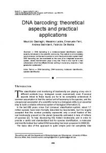
tire scheme /see fig. I / z I~) for given value 2)

v~

the Infimal Problems

are solved and the

Q ( vk) is sent to Supremal Problem (SP)

on the base of the knowledge of /i

IP

=

^i Q ( v k) ,

I ,... ,N /and eventually some other informatiens from IP/

the coordinator chooses new value of coordination variable k+1 (~) v , sends it to IP and step I) is repeated unless Q = = min v£V

Q ~v) ,

in which case the ooerdination is finished.

s

;y

IP !

_

J " • •

[

IP/V

Ft'g. I The generul scheme Ok informu~t'on flow in lhe Pr(~l Melho~

402 1.3.

General properties In this section we will summarize the main properties of the

Primal Method. Definition

I

The problem ~I) is coordinable by the Primal Method if there exists and =~

v

~

V

such that

s

x0 = ~ ( m , v '" Q ° ~ m ~

,

v) and

with given and fixed

Q (v)=

min vEV

Q(v

)

s is the solution of (I) , where mv ,

i

=

I,..~,N

m,

=

are the solutions of

IP

v .

Remark It should be noted that if problem (1) is coordinable by the Primal Method then for some solution

,

of

2

we have

m~

= m.

Theorem 1 of problem ( 1 ) exists amd ^i that for every v £ V there exist the solutions m of IP. o v Then problem {I) is coordinable by the Primal Method. Let us suppose that the solution

The proof is given io [12j

x

[16]

It should be noted, that the infimal problems may have net s o l u t i ~ for every

vEV o

in the case when there exists the solution

( I ) or equivalently the solution (m, v) of ( 2 3

x

of

/see eg. [12j /.

Since the optimization is to be carried out by numerical methods the following property of the Primal Method is quite important. Theorem

2

If any local minimum of problem (2) is a global minimum of this problem then every local minimum of the of

SP

is also a global minimum

SP. Moreover if problem (2) has a global minimum then the

SP

has

also a global minimum.

proof is given in Eli , L121 . In

~

it has been shown that the infimal problems

IP

may have

403 local minima even when problem (2) has no them an4 so the more detailed conditions have to be examined. Definition

2

We say that mapping

R :

A D

A

/A,B - linear spaces / is concave on cone

S C B

if V

x I, x 2

- (I

~

Ao

o

~ A

B with respect to the convex

o

and

V

~6[0,I]

+ ,(9xi +(I

x2) s

,Theo,rem 3 Assume that (i)

~io '

V1

are convex, closed sets,

(ii)

yie '

Z

are

convex, closed cones,

Mi v

are compact for every

o

(iii) the sets

v ~ V

o

,

(i%)

the functionals

Qi

(v)

Mix V, 0 the mappings

are continuous and concave on

respect to

Gi yio '

and concave on ~en

are lower semi-continuous and convex on

i = I,°o.,N

V

i = I,.o.,N ,

Mi

X V

with

and the mapping ~ o is continuous

with respect to

Z . o

sets

M i are convex for every v g Y , set V is convex and v o o closed, functional Q (") is convex ana finite on V . o If, moreover, the set W has the nonempty interior then V has also o the nonempty interior and ' 'V v E int V sets M i have the nonempty o v interiors. The proof is given in

[11]

, ~2] .

In the following sections we will investigate the more detailed properties of the Primal Method, especially important for numerical applications.

404

2.

Theoretieal~rqperties Some of the

SP

of the

Supremal

'

Problem

properties have been just summarized in Theorem 3o

In this section we will discuss two questions. representation of sets

Vo,

Vs

One is about the

and the problems connected with it;

the ether is about differentiability properties of the index

SP

performance

Q .

2.1. Representation of the feasible sets

V , V . o s Usually, when numerical methods of optimization are applied to a

given problem, they require analytical expressions or at least some subroutines for the feasible set representation. we meet this problem because the now specified only by C7).

SP

When solving the

feasible set

Vs

has been up to

We may of course assume that the set

is known explicitly as well as the constraint mapping further considerations we will for simplicity take

SP

T .

V I = V.

VI

So in Bat there

is the serious problem with set

V • It is so far defined implicitly o this definition does not give us any analytical representat-

by (5) ; ion of

V

and the knowledge of such representation is even more

o

essential than in standard mathematical programming problems just because for

v ~ Vo

the infimal problems are not well defined.

In many cases it is possible to obtain the analytical expression for

V

/see [3] , [IO3 , [I~ /. This means that we oau find / when o the decomposition is being made /the mapping h: V - - > R ~ , ~ ~ such that

To il!~strate this idea we give a simple example:

let

¥ = R 2 and

suppose that we have two infimal problems in which there are the local cons traints

I> ilm I iJ .< v l 2) ji m2H where

m

I

, m

2

v = {vl v2}

2

belong to Bamach spaces

MI

, M

2

.

Suppose also that there is one supremal problem constraint vI

+

v2

%

a

,

a

>

0.

405

In this ease the mapping and

Vo = ~ v ~ R2

..

v1~

h

has the following form:

0 ,

v2 ~

O~

=

R 2+

while Vs In a general case it may be not possible to decribe set in (8) °

V~ o

as

We may only to prove the following theorem:

Theorem 4 Assume that: (i)

yi /i = I,...,N/ are Banach spaces and yi ~ y i o

M i are convex sets, o Gi (iii) mappings are concave on

yi are convex cones, 9

(ii)

yi o 7 (iv) for every v • V

Mi ~ o

V

with respect to convex

cones

are compact and Then

v 6 V

Gi( • ,

Gi(M~ , v) are compact /e.g. when

#

9

v) are continuous /.

if and only if

o

max

the sets

Zi ,

Gi(m i

v)

(9)

o for every

hi E A

i

, where

Ai

Ai

1

The proof of the above theorem is given in [1 2] . Theorem

4

shows that set

V

is, in a general ease, determined o by infinite number of inequalities (9) • If yl are separable Banach spaces then it is sufficient to take only countable number of inequalities (9) •

However it is still troublesome to consider all of them.

There is another problem connected with maximum operation performed in (9) mi max i - since that maximization has to be carried on for E Me ~/ By we denote the value of linear continuous functional a ~ X~ on b ~ X /X-Bauach space, X~-dual space tc If X C X and X is a cone then by X ~ we denote cone o o o conjugated to X . o

406

every

v

of interest.

required, namely when

There is one important case when this is not G i ~ m i,v) =

G li(m i) + G2i (v~ .

In some cases

/ ~12] / it is possible to prove that we can take only finite nmmer of

inequalities C9) • Summarizing then there are essentiatly two main problems connected with set

V • First of them is that we de not know in general the o analytical representation of this set. The second is, that for v ~ V °

the infimal problems are not well defined /their feasible sets are empty/ and so it is not possible to apply for solving the

SP

for

example exterior penalty function numerical methods for comstrained problems.

In section

3

we will describe some methods which may prove

capable of handling in some eases the difficulties mentioned above. 2.3. Differentiability properties of the

SP

performance index

Q .

It is very well known that differentiability properties of performance index are of extreme importance for application of numerical methods of mathematical programming. In this section we assume that

M i, V, yi, Z

are reflexive

Bamach spaces, Y

Z are closed convex cones, mappings G i, T are o Pr@chet differentiable and concave with respect to yio t Z * o Q is assumed to be convex on ~ x V and bounded on every bounded set in

M

x

V.

Mi

are convex, closed sets and

W

is bounded,

satisfying the Slater's regularity condition / ES~ /. Then we can prove the following important theorem. Theorem If

M i = M i for o performsmce index Q

i = I,...,N has in

vO

of the form,"

The elements at

~ V then the SP o o subdifferential ~ Q C v O) on

VI/o

N

:

Q (-)

stud v

P = qV + o

(10) i =1

Vo

p ~ ~ Q ( r e ) are called subgradients of v

= v o.

407

where h i , i = I,...,N mv c

and the /possible/ solution of infimal problems

= (my ' ' " ' ~ N ~ satisfy the conditions, o o %3

+

=

v

o

v o

o

"i

(II) o

~3~

- yi~,

i = 1,..°,g

~m i v

- Fr@chet derivate with respect te

and

of

o

H

i v

m

G i in the p o i n t ( m^i v , v° ) t e

- Fr@chet derivative with respect to o

of

i

i G

in the

c _i point._v

%) t

v o

e q^im ff v o

~m i

Q ( m^v

'

I73

To)

o

- subdifferential of Q with i respect to m /o - subdifferential of Q with

o

@

respect to v /.

The proof is given in [12] . Lemma If

I v

~ int V then the subdifferential set (10) of the above o o theorem is nonempty, convex and weakly compact. The lemma can be proved directly / [12] /, but the result cam be also obtained from theorem

3

since convex and finite functional has

the nonempty, convex and weakly compact subdifferential / in Bauach reflexive space/ in every interier poimt of its d o m a i n / e.g. [6] /.

Remark It can be seen from Theorem for

Q

5

that the sufficient conditions

to be Gateaux differentiable at

v

g ¥ are: o .o uniqueness of the infimal problems solutions m~ / due for example o

408

to the strict convexity of

Q/,

existence and uniqueness of ~ i

A

satisfying (I I) and Gateaux differentiability of

Q

with respect to v

at the point ~m~ , re) • o Theorem

5

can be generalized / [I 2] / to the case when

convex closed cones with nonempty interiors. conditions for

Gi

M i are o The differentiability

may be rejected / [I 2] / if

yi = R~.~ o + In this case the assumption about concavity of

yi

are finite

dimensional Euclidean spaces and

Gi

may be weakened to

the quasi-concavity assumption / [11] /. It may be there a considerable difficulty if /~Ye

- boundary of

V

o

v g ~V o o / since in this case it may happen that

(vo) is empty/[12J/. The above theoretical results form a basis for the developed in the next section.

SP

algorithm

They also show us the complexity of

problems connected with applications of the PTimal ~ethod.

409

3.

The

ST

coordinatiou algorithms

The Primal Method requires in a natural way the coordination strategy for solving the

SP

being some numerical minimization

procedure /see [2~ , [12] /. which the solution of the

Theorem

SP

I

gives the conditions under

exists and Theorem

there are not local minima in the

SP

2

quarantee

that

when there are net local minima

in the decomposed optimization problem°

This fact is very important

for the application of any minimization procedure as the coordination strategy.

However there still is a question what minimization

procedures could be applied.

The problems connected with set

differentiability properties of

and e which have been discussed before

Q

V

make it clesy~ that we cannot just use standard procedures of mathematical programming.

So some special algorithms should be developed.

There is moreover one additional and a very important demand which ought be satisfied by these algorithms.

They should need the least

possible number of the goal function evaluations to reach the solution since every evaluation of

Q (v) requires the solving of all i~fimal

problems which may be a very time consuming task. In this section we will describe the algorithms for finding the best direction of improvement for

Q

at the points belonging to

We will also outline three algorithms for solving the of them is based upon the idea of subdifferential of

SP. Q ,

V e.

The first the

two

others are heuristic algorithms capable to handle the most serious problems connected with coordination in the Primal ~ethod. = yi We assume everywhere in this section that ¥I V , ~ V

are

finite dimensional spaces and all the assumptions made at the beginning of section 2.3

held.

We assume also that mapping

T

is Gateaux

differentiable. 3.1. The best direction of improvement In every point

v

G V

o

in which the subdifferential of

nonempty and compact / and so by lemma of

I

in every interior point

V / we can compute the best direction of improvement for

This direction is defined as follows:

Q

Q .

is

410 Q ( v~ O*/

D A

(12)

s

subject to v+

s gV

o

~d

for

< v t k (v) ~ o>>~o where

tk

lrEK(v)=fk:

tk(v) = 0}.

is

k-th component of T = ( t I .... t ) nz n tk: V---~ R and Z = R z o + "

DQ (v~ s) is connected with % Q (v) in the followimg way /see [ 6 ~ / .

D~ (v: s) = m=

i

i

corresponding to nonactive constraints are set to zero and

J

v

Q(;v v)+ H+[ >ioo

i m

mv

i

- yi~-

A

o

R ~ +

yi = o

/we assume here that

/

So if some procedmre for solving the search in any given direction linear programming problems if ement.

s

SP

is carrying on the

then it may be checked by solving N s

is still the direction of improv -

This may save some computational effort for solving the /non-

linear/ infimal problems in the ease when ion of improvement for To compute (12) , (14) .

sv

s

is no longer the direct-

~ +

we have to solve in general the min max problem

However if the assumptions mentioned above are

satisfied and (14) is the linear programming problem we can transform

/see [8] , [11] /the rain max prob1~ 0 2 ) , 0 D

to the following

linear programming problem /ref. [11]/if in space

V = Rn v

we define

the norm as

vH = maxlvil i

= I,°o.,~

v N

+

Q (~, v), s> +

min

i=I

] 0+)

smbj oct to i Mi z 6 ,

+to++i

i = I,...,N

~< ~oiv s / ~i'° ~iv

m

-I

m

~< sj ~ I

- Jacobiams cf active constraints only/

, j=1,...,~ v

and

~ o

~or k~K(v).

412

Obviously, we are interested only in finding

s

v

solving the

above problem. There are however some difficulties which can be encountered when solving problem (15) .

First, it may happen, if the infimal problems

are not solved absolutely correctly, then the problem (15) has an unbounded solution.

Second, the application of (15) will require

considerable exchange of information between the which may be sometimes nondesired,

SP

and the

IP-s

Besides it the problem (15) has to

be solved only in such points of V

in which Q is not differentiable o /the measure of such interior points of V is zero- see [15J /. o If Q is differentiable at v g V we can find the gradient of o

(v) / in mother ways/ which may be simpler/, eq. by solving the eqs. (11) to find

hi

and substituting to (10) .

In the sequel

we will describe the method for finding V Q (v) based on the shifting penalty function method used for solving the infimal problems. Summarizing then is seems that the following scheme could be preferable in some eases /e.g. in the coordination for improvement 9f real processes [3S , [12] /: (i)

check by solving (14) if the direction the

s

of search used by

SP

procedure is indeed the direction of improvement of Q; k+1 k if it is, then solve the imfimal problems for v = v + ~k s /where ~k

is some specified positive number/ and repeat (i) |

if not, then go to (ii) (ii)

choose the new direction

s

computations required to find

or /if necessary/ perform the s

v

/ e.g. by solving (15)/.

hen go to (i) It seems that the above scheme should be further investigated.

3.2.

The subgradient algorithm We will discribe now shortly the algorithm, which can be used

for solving the are fulfilled and

SP. V

We assume here that the assumptions of theorem 5 is Euclidean space.

Suppose at first that

V

= V = V /this assumption will be s o partially relaxed later/, and that some sequence ~ k ~ of real posi tire

413

numbers is given having the following properties: OO

~d

%~o ÷

~

~

=+=

k=1

the subgradient algorithm generates

Starting from any point v ° ~ V O k the sequence v according to: k+1 v

k =

k

v

- ~Ik

P

'

(16)

k = 0,I,..~

where

pk ~

(k), k

! 0

if

p

i ~k

if

p~

=0

,~ o

Convergence ~ of the above algorithm has been proved in [IJ . It should be noted that after solving the infimal problems we can k rather easily compute some p G B Q ( J ) , but algorithm (16) is supposed to be very slow because of the proporties of sequence ~ k l

"

Remark If

V

C ¥ S

= V 0 ~_.

then the above algorithm has to be modified•

-~

After computing ~ t l ) f r o m onto

V

(16) it i s necessary to project

to generate the new point

vk+1

of ~ k 1

S

3.3.

"¢~'1)'

•

The local penalty ftmction algorithm. As we have mentioned above there is a need to develop the practic-

al method for finding V Q (v) whenever it exists•

It has been shown

in [8~ that it can be done by application of the shifting penalty function method te solve the infimal problems•

~__ ~ O

t

~ =(_~

~eoe~

We assume here that

-,~ J.~(~ c. ~ ,~ ..,~ (~ ~

~e

t

,~}

=

Y t

i=I The penalty /shifting/ function method means the repetive minimization of the following function /we consider the

problem/:

i-th infimal

414 it i i K~m,v,-,~)i)=

Qi

mi, v

+

~J

I

i i (i,v ) + O~) •

07)

wj (gj j=1

• wherej = 1 , . . . , ~ i

i

,

wj~

(0, 4

.)+ o J

0 are the penalty coefficients sad

are penalty shifts. Suppose that at point

m

- the solution of

v

i-th imfimal problem-

the following comditions are satisfied: m

K i ( mv ' v ; w

i

i(-i

v) g o

5-~'

~

j=1 '

~ I O'= 0

=

'""

0

08)

ni g

for Jr Ji-v-j' ~Jif(v)=[j: g~(miv , v)

o}

Then it may be shown, that

~

= ,ij ~ ij / j = I,..., ngi / is the sol~ion of egs. (11).

So if the Lagrange multipliers are determined uniquely then they cam be directly computed from the penalty fmnetion° Prom the above result and Theorem

" v)÷ ~ v~i(v) = vv Qi(~;, .e~ =

~v

j=I

5 i t fellows that

i ~iv, v) = ~i Vv %( J

^i , v) + Qi ( mv j=1

If in the point

v

exists

09) (v) then it can be computed according

~o (19) =:

V~(v) = ~v~i(v)

(20)

i=I The algorithm presented in this paragraph is designed in the way to avoid the difficulties connected with set

V

o

/ r e f . [8] / .

The shifted penalty function method has the property that in most i cases the penalty coefficients w. do net hate to be increased to infinity to find the solution

mvi~.

They will of course increase to

415

infinity if set

Mi

is empty.

V

In our algorithm we use the modified two-level optimization problem.

The aim of this modification is to obtain the

unoonstraint minimization problem.

SP

being the

The modification is achieved in

the following way: if during the solving of the infimal problems for given

v • V

by the shifted penalty method (I) the routine termination criteria are satisfied with

wi ~ w max

or

(2) some of the penalty coefficients then the

SP

wt become greater than J functional value is set as Ki( m L

v,

w

w

~i)

V ~

i=1

,

,,ith

;i

being t h e a c t u a l v a l u e s o b t a i n e d when s o l v -

V

ing the infimal problems. V Q (v) is then computed according to (19) , (20) and nsed by some coordination strategy /e.g. by the conjugate gradient method/. The local penalty function algorithm / ~ i g . ~ is as follows: (i) Set the initial values /with r e a s o n a ~ great

w /, o (ii) Solve the modified two-level optimization problem. ~k ^k After this problem is solved we have v t m . (iii) If

~k 6 V

in the sense that for some specified

~>0

O

i gj(m k, ;k).< E, j = I,...,nyi -k v

then we assume that

If i

w_ J

Sk ~

VO / i t

;

I,...,N

i

is the solution of our

SP.

i s some i n f i m a l problem i s stopped because

gets greater than

w

/then set max

and go to Cii) with

~k

~k

m , v

w

~

w

max

+ ~ max

treated as the initial point there.

~ i s algorithm have been tested and it have appeared that it can behave quite well and /as usual in numerical applications/the success depends heavily on the skill with choice of the routine parameters for the shifted penalty function method and the point

4. I. of this paper/.

SP

procedure /see

416

k~O

":'1 L_

w,,~,.

C22)

A

where and

q q~ ~

is the optimal value of original problem performance idex q~

are optimal values of modified problems.

(22) gives the lower and upper bounds for ble for numerical applications.

q

The relation

and thus may be valua-

419 4.

0omputational results and oonclussion8 Some of the algorithms described above has been tested om the

following decomposed nonlinear programming problem: i/

the infimal problems:

1° rain [ Q l ( m I , v) 1 m

= 100 (m 1 - Vl ) 2 + (1 - v 1) 2] J

subjeet to

1

m ~

NIl

1

v =I

ml~ R :

,40 ./m 2 +V 1l ' O v0.04 , (m1~

0 t

Q

2.

mi. [ J ( . ~ , v) -- O° v~ + v~ ) ~ ÷ ~(m~ - '~)~ ~ + m

2

+ ( v 1 - 2 m ; ) 4 + I0 ( v 2 - m~)4.J subj oct to

m

v

'-"I-

+-=

- o.oo~

o

.

.in[Q3c°3 .)= oo(.3 (*2 3)2 + 0

21

m3

subject to m3~ M3v = I m3~ ii/

R :

m

+ v2

o.53

~< O, - m 3 ~ o

the supremal problem IILtn{Q(V) = 7 subJect to vE V ={v e

QI(v) +

E R2 : v E ¥o ' v2 ~ O~

where

vo={v~2

_ vl -0,04~