RLE Technical Report No. ... Massachusetts Institute of Technology ..... Spaces ae denoted with the blackboard bold math font, e.g., Rn. The symbols for ..... the techniques are applied in top-down fashion (e.g., integration, nonlinear solution,.
Theoretical and PracticalAspects of Parallel Numerical Algorithms for Initial Value Problems, with Applications RLE Technical Report No. 574
Andrew Lumsdaine
September 1992
Research Laboratory of Electronics Massachusetts Institute of Technology Cambridge, Massachusetts 02139-4307
Theoretical and PracticalAspects of Parallel Numerical Algorithmsfor Initial Value Problems, with Applications
RLE Technical Report No. 574
Andrew Lumsdaine
September 1992
Research Laboratory of Electronics Massachusetts Institute of Technology Cambridge, Massachusetts 02139-4307
This work was supported in part by IBM Corporation, in part by the Defense Advanced Research Projects Agency under the Office of Naval Research grant N00014-91 -J-1698 and under the National Science Foundation grant MIP-88-14612, and in part by an AEA/Dynatech faculty development fellowship.
ii
Theoretical and Practical Aspects of Parallel Numerical Algorithms for Initial Value Problems, with Applications
by Andrew Lumsdaine Submitted to the Department of Electrical Engineering and Computer Science on January 2, 1992, in partial fulfillment of the requirements for the degree of Doctor of Philosophy
Abstract Theoretical and practical aspects of parallel numerical methods for solving initial value problems are investigated, with particular attention to two applications from electrical engineering. First, algorithms for massively parallel circuit-level simulation of the grid-based analog signal processing arrays currently being developed for robotic vision applications are described, and simulation results presented. The trapezoidal rule is used to discretize the differential equations that describe the analog array behavior, Newton's method is used to solve the nonlinear equations generated at each time-step, and a block preconditioned conjugate-gradient squared algorithm is used to solve the linear equations generated by Newton's method. Excellent parallel performance of the algorithm is achieved through the use of a novel, but very natural, mapping of the circuit data onto a massively parallel architecture. The mapping takes advantage of the underlying computer architecture and the structure of the analog array problem. Experimental results demonstrate that a fullsize Connection Machine can provide a 650 times speedup over a SUN-4/490 workstation. Next, a new conjugate direction algorithm for accelerating waveform relaxation applied to the semiconductor device transient simulation problem is developed. A Galerkin method is applied to solving the system of second-kind Volterra integral equations which characterize the classical dynamic iteration methods for the linear time-varying initial value problem. It is shown that the Galerkin approximations can be computed iteratively using conjugate-direction algorithms. The resulting iterative methods are combined with an operator Newton method and applied to solving the nonlinear differential-algebraic system generated by spatial discretization of the time-dependent semiconductor device equations. Experimental results ae included which demonstrate the conjugate-direction methods are significantly faster than classical dynamic iteration methods. The results from both applications are encouraging and demonstrate that for specific initial value problems, the largest performance gains can be achieved by using closely matched algorithms and architectures to exploit characteristic features of the particular problem to be solved.
111
iv
Thesis Supervisor: Jacob K. White Title: Associate Professor Thesis Supervisor: John L. Wyatt, Jr. Title: Professor
To Wendy, with all my love
V
vi
Acknowledgments It was my profound privilege to have two supervisors, Prof. Jacob White and Prof. John Wyatt, directing the research contained in this thesis. Not only did they direct my work to ensure its quality, but, more importantly, they taught me how to direct myself. I must add that having two supervisors, especially two of the caliber of Profs. White and Wyatt, has benefited me far more than twice as much as having a single supervisor. I am grateful to several fellow graduate students without whose help I never would have finished the work in this thesis. Foremost I must acknowledge the extensive assistance I received from Miguel Silveira. Throughout our three-year relationship, we collaborated on several large projects, in particular SIMLAB and CMVSIM. These programs would never have been completed without him and would certainly not be as elegant without the refinement they obtained as a result of our constant wrangling over details. I worked very closely with Abe Elfadel on several vision related projects. Abe was always a knowledgeable resource for any sort of questions I had of a theoretical nature - and there were a lot of them. Mark Reichelt gave a large measure of his time in providing me with access to his WORDS program and in helping me with the implementation and experiments for the waveform conjugate direction methods. Bob Armstrong was always available when I needed a software or hardware guru - he developed and provided the lab with a variety of useful tools, many of which were used in the preparation of this document. I would also like to acknowledge Thinking Machines Corporation and Rolf Fiebrich for the generous contribution of their resources, Prof. Zhengfang Zhou for several helpful discussions, the MIT Vision Chip group for providing the motivation for the work in Chapter 3, and all the other students and faculty in the VLSI CAD group for their support and friendship. Finally, completion of this thesis would not have been possible without the love and encouragement I received from my family, especially from my wife Wendy. I thank her for being so patient during the course of my graduate program and for supporting me financially, emotionally, and spiritually during that time. Thanks also to my parents, Edward and Monika Lumsdaine, who, on top of all the support they have given me over the years, found the time to proofread this thesis. This work was supported by a grant from IBM, the Defense Advanced Research Projects Agency contracts N00014-87-K-825 and MIP-88-14612, the National Science Foundation, and an AEA/Dynatech faculty development fellowship.
vii
viii
Contents 1 Introduction 1.1 Initial Value Problems ......... 1.2 A Circuit Simulation Problem ..... 1.3 A Device Simulation Problem ..... ................ 1.4 Overview. 2
3
1 1 3 4 5
................ ................ ................ ................
Review of Numerical Techniques 2.1 Introduction .............. 2.2 Linear Solution Methods ....... 2.2.1 Direct Methods . . . . . . . . . 2.2.2 Relaxation Methods ..... 2.2.3 Conjugate Direction Methods 2.3 Nonlinear Solution Methods ...... 2.3.1 Newton's Method ....... 2.3.2 Nonlinear Relaxation ..... .. .. 2.3.3 Inexact Newton Methods .... 2.3.4 Matrix-Free Methods ..... . . 2.4 Integration Methods .......... . . 2.5 Waveform Methods .......... . . 2.5.1 Waveform Newton Methods . . . . 2.5.2 Waveform Relaxation Methods . . 2.5.3 Inexact Waveform Newton Methods 2.6 Parallel Techniques ............ Parallel Simulation Algorithms 3.1 Introduction. ............ 3.2 Problem Description ....... 3.2.1 Motivational Problem . . . 3.2.2 General Array Description 3.3 Numerical Algorithms ...... 3.4 Implementation ........... 3.4.1 Data to Processor Mapping 3.4.2 Device Evaluation ..... 3.4.3 Linear System Solution . . .
.. . . . .
.. . . . . 0
0
·
............ ............ ............ ............ ............ ............ ............ ............ ............
0
. . . . . . . . . . . . . . . .
. . . . . . . . . . . . . . . .
. . . . . . . . . . . . . . . .
. . . . . . . . . . . . . . . .
. . . . . . . . . . . . . . . .
. . . . . . . . . . . . . . . .
. . . . . . . . . . . . . . . .
. . . . . . . . .
. . . . . . . . . . . . . . . .
. . . . . . . . .
. . . . . . . . . . . . . . . .
. . . . . . . . .
. . . . . . . . . . . . . . . .
. . . . . . . . .
. . . . . . . . . . . . . . . .
. . . . . . . . .
. . . . . . . . . . . . . . . .
. . . . . . . . .
. . . . . . . . . . . . . . . .
. . . . . . . . .
. . . . . . . . . . . . . . . .
. . . . . . . . .
. . . . . . . . . . . . . . . .
7 7 7 9 9 11 13 14 14 15 16 16 17 18 19 19 20
. . . . . . . . .
25 25 26 26 27 31 34 35 36 36
ix
--------
CONTENTS
x
3.5 3.6 4
5
3.4.4 Grid Boundaries ............. Experimental Results .............. Conclusion. ....................
Conjugate Direction Waveform Methods 4.1 Introduction. ................... 4.2 Description of the Method ............ 4.2.1 Operator Equation Formulation ..... 4.2.2 Classical Dynamic Iteration Methods . . 4.2.3 Accelerating Dynamic Iteration Methods 4.2.4 Hybrid Methods for Nonlinear Systems . 4.3 Device Transient Simulation ........... 4.4 Implementation .................. 4.4.1 Main WR Routine ............ 4.4.2 Operator Waveform Product ...... 4.4.3 Inner Product .............. 4.4.4 Initial Residual ............. 4.5 Experimental Results .............. 4.6 Conclusion. .................... Conclusions
.............. .. .. .. . . .. .. .............. .............. .............. . . .. .. . . .. . . . .. . . . . . . . . .. . . . .. . . . . . . . . . . . . . . . . . . . . . . . . . .
. 39 . . . . . . . . .40 . . . . . .. . .50
. . . . . . . . . .
. . . . . .. . . . . .
. . . . . . . . . .
. . . . . . . . . . .
. . . . . . . . . . .
. . . . . . . . . . .
.. . . . . . . . . . .
. . . . . . . . . .
. . . . . . . . . . .
53 53... 54... 55... .56 .57 .65 .67 .69 .69 .71 .76 .76 .77 .80
83
List of Figures 2-1
A (non-exhaustive) taxonomy of methods for solving IVP's .......
.
8
Grid of nonlinear resistors . ......................... A single subcircuit, shown here as a multiterminal element, and a grid constructed of such elements ........................ .......... . 3-3 Example graphs for circuits C and C.................... ......... . 3-4 Decomposition of the example circuit shown in Figure 3-1 ...... 3-5 Mapping of subcircuits to processor grid ................... 3-6 Definition of P .............................................. 3-7 Example separation of a subcircuit into sub-subcircuits . .......... 3-8 Linear resistive grid .............................. 3-9 Mead's Silicon Retina ........................................ . 3-10 256 x 256 image of the San Francisco sky line . ............. ...... . 3-11 Output images produced by ,-continuation network ......... (a) Output produced by /-continuation network, 3 = 0.......... (b) Output produced by fl-continuation network, = 2 x 10⁴ .. .. . . (c) Output produced by -continuation network, = 1 x 10⁶...... . 3-12 Output images produced by Af-continuation network . ........... (a) Output produced by Af-continuation network, Af = 1......... (b) Output produced by Af-continuation network, Af = 1 x 10- 3. .. (c) Output produced by Af-continuation network, Af = 3 x 10- 5 . . .
27
3-1 3-2
4-1 4-2 4-3 4-4 4-5
Convergence comparison between WR and WGCR for eigenvalues {1,10}. Convergence comparison between WR and WGCR for eigenvalues {1,100}. Convergence comparison between WR and WGCR for eigenvalues {1,1000}. Convergence comparison between WR, WRN, WGCR/WGMRES, and WCGS for jD example . . . . . . . . . . . . . . . . . . . . . . . . . . . Convergence comparison between WR, WRN, WGCR/WGMRES, and WCGS for kD example ............................
xi
28 30 32 35 38 42 43 45 46 48 48 48 48 49 49 49 49 65 66 66 79 79
xii
LIST OF FIGURES
List of Tables 3-1 3-2 3-3 3-4 3-5
Comparison of direct, CG, ILUCG, CGS, and ILUCGS linear system solvers. Experimental result: Linear circuit grid . ................. Experimental result: Nonlinear circuit grid ................. Experimental result: Mead's Silicon Retina, constant input image ..... Experimental result: Mead's Silicon Retina, random input image .... .
34 42 44 45 46
4-1
Comparison of WR, WRN, WGCR, WGMRES, and WCGS ........
78
xiii
xiv
LIST OF TABLES
List of Acronyms CD CG CGNR CGS CM DAE GCR GMRES GJ GS ILUCG(S) IVP KCL KVL MICCG MIMD MOS MOSFET NLR ODE PDE QMR SIMD VLSI WCGS WGCR WGMRES WN WR WRN
Conjugate Direction Conjugate Gradient CG Applied to the Normal Equations Conjugate Gradient Squared Connection Machine Differential Algebraic Equation Generalized Conjugate Residual Generalized Minimum Residual Gauss-Jacobi Gauss-Seidel Incomplete LU Factorization Preconditioned CG(S) Initial Value Problem Kirchoff's Current Law Kirchoff's Voltage Law Modified Incomplete Cholesky Factorization Preconditioned CG Multiple Instruction, Multiple Data Metal-Oxide-Semiconductor MOS Field Effect Transistor Nonlinear Relaxation Ordinary Differential Equation Partial Differential Equation Quasi-Minimal Residual Single Instruction, Multiple Data Very Large Scale Integration Waveform Conjugate Gradient Squared Waveform Generalized Conjugate Residual Waveform Generalized Minimum Residual Waveform Newton Waveform Relaxation Waveform Relaxation Newton
xv
xvi
LIST OF ACRONYMS
List of Symbols Vectors Members of a vector space are denoted with the bold math font, e.g., . The vector space in question may be R , or a function space. Components of a multidimensional vector are denoted in the plain math font, with the appropriate subscript, e.g., xi. If the vector space is additionally an inner product space, the inner product of x and y is denoted by (, y). Constant vectors are sometimes indicated with a subscript, e.g., xo. The symbols for some particular vectors used in this thesis are: b Right-hand side (as in Ax = b).
e Error. The elementary basis vectors for Rn are denoted el,.. ., en. p Search direction. r Residual. Matrices Matrices are denoted in upper-case with the bold math font, e.g., A. Components of a matrix are denoted in upper- or lower-case with the plain math font, using the appropriate subscript, e.g., Aij or aij. The algebraic or Hermitian transpose of a matrix is denoted with a superscript t, e.g., At. The identity matrix is denoted by I. Operators Operators ae denoted in upper-case with the script font, e.g., A. Spaces Spaces ae denoted with the blackboard bold math font, e.g., Rn. The symbols for some particular spaces used in this thesis are: L 2 ([0, T], Rn) Function space of square-integrable functions (in the Lebesgue sense) mapping from the interval [0, T] to Rn. N Set of natural numbers, i.e., {1,2,.... Rn n-dimensional Euclidean space.
xvii
LIST OF SYMBOLS
XVlll
Miscellaneous The following is a brief description of other miscellaneous nomenclature: k
The superscript k denotes the kth iterate of the associated quantity, e.g.,
xk is
the kth iterate of x. The superscript k is the usually used for iterates with a linear iterative procedure, whereas the superscript m is usually used for iterates with a nonlinear iterative procedure. Indexing generally begins from k = 0. Occasionally, the superscript is also used for exponentiation, but those cases will be clear from the context. cl A Closure of the set A. ess.sup Essential supremum. V
Gradient of the function q5.
I(-) Lower bound complexity. O(.) Upper bound complexity.
1
Introduction 1.1
Initial Value Problems
Many interesting applications can be modeled as an initial value problem (IVP), e.g.,
F(z'(t), x(t), t) = 0 x(O)
=
0
~~~~~~~~(1.1)
= z0
where z(t) E Rn and F: R 2n+ -* R". Here, (1.1) can describe an IVP for an ordinary differential equation (ODE) system or for a differential algebraic equation (DAE) system. It is assumed that The function F is such that the solution z(t) exists and is unique on a simulation interval of interest, say, t E [0, T], and that the initial condition is consistent for the DAE case. In general, an analytic solution to (1.1) cannot be found, so the problem must be solved numerically. With the typical approach, (1.1) is first discretized in time with an integration method. Since DAE and stiff ODE systems require the use of implicit integration schemes, the time discretization will generate a sequence of nonlinear algebraic problems which are solved with an iterative method, usually a modified Newton method. The sequence of linear algebraic systems generated at each iteration of the nonlinear solution method are then solved with Gaussian elimination. The above process is the "implicit-integration, Newton, direct method" canon and forms the basis for most general-purpose codes for solving large-scale IVP's [1]. The standard approach has two computational bottlenecks (which bottleneck will dominate depends on the particular problem):
* Function evaluation -
computation of F(-) and the associated Jacobian JF(-). The cost of evaluating JF grows with problem size and with the degree of coupling. 1
2
CHAPTER 1.
INTRODUCTION
For densely coupled problems, evaluating JF costs O(n2 ) operations; for sparsely
coupled problems, the cost of evaluating
JF can
be as low as 0(n).
* Linear system solution - solving the linear system at each iteration of the nonlinear solution process. The complexity of direct elimination methods for solving systems of equations is polynomial in n, typically from O(nL5 ) for sparse problems to 0O(n 3 ) for dense problems.
When using the standard Newton method, the function evaluation and the linear system solution are performed at each iteration of each nonlinear system solution at each timestep. However, certain modified Newton methods recalculate the Jacobian only at certain intervals (e.g., every third Newton iteration) [2], thereby reducing the work required, although not the complexity, by a constant factor. Efforts to improve the computational efficiency for numerically solving IVP's focus on improving the efficiency of the function evaluation and the linear system solution. These efforts fall into two general (overlapping) categories: algorithmic improvement and hardware improvement. For example, one could use an iterative method for the linear system solution, or implement the solver on a vector or parallel processing machine. For some problems, such an approach might be highly effective, but for other problems, such an approach might be a disaster. It seems that general-purposecodes for solving IVP's must follow the "implicit-integration, Newton, direct method" canon because such codes are written to be able to reliably handle the largest possible class of problems. However, this formula can be quite limiting for specific problems that can benefit from the application of more specialized algorithms. Therefore, the following observation is made, which is the theme of this thesis: For specific initial value problems, one can achieve the largest performance gains by using closely matched algorithms and architecturesto exploit characteristicfeatures of the particular problem to be solved. This thesis will examine methods for solving two initial value problems from electrical engineering - a circuit simulation problem and a device simulation problem. The attacks on these problems will be two-fold. First, methods suitable for implementation on parallel machines will be developed. Second, it will be attempted to exploit the problems fully through the use of sophisticated numerical techniques.
1.2.
3
A CIRCUIT SIMULATION PROBLEM
1.2
A Circuit Simulation Problem
The nodal analysis formulation of the circuit transient simulation problem is described by + i (v(t)t) = dq (v(t)t) Tt~~~~~~ v(0)
=
0
(.2) (1.2)
v0
where v(t), q (v(t),t), i (v(t),t) E Rn are the vectors of node voltages, sums of node charges, and sums of node resistive currents, respectively, and n is the total number of nodes in the circuit. Numerical techniques for solving (1.2) are very well developed - for all practical purposes, the general circuit simulation problem has been solved [3, 4]. Programs like SPICE [5] or ASTAP [6] -
which follow the "implicit-integration, Newton, direct method"
approach to solving (1.2) -
are capable of simulating virtually any circuit, given enough
time. Unfortunately, for some types of circuits, "enough time" is too much time for simulation to be a practical part of a circuit design cycle. Robotic vision circuits [7, 8] form one such class of circuits which are intractable for standard analog circuit simulators such as SPICE or ASTAP. The vision circuits are necessarily very large and must be simulated at the analog level (i.e., one cannot perform simulations at a switch or gate level as is commonly done with very large digital circuits). Standard analog circuit simulators are not able to handle vision circuits simply because of their immense size, since the computation time for these simulators grows super-linearly with the size of the circuit. This super-linear growth is particularly pronounced for vision circuits because their structure produces a Jacobian matrix that generates much more fill during Gaussian elimination than do generic circuits having the same number of nodes. Although the structure of the vision chips is disadvantageous for a direct-methods solver, it is advantageous for other algorithms and for certain parallel architectures. In particular, the regular structure of the problem implies that the simulation computations can be accelerated by a massively parallel SIMD computer, such as the Connection Machine®[9]. Moreover, the coupling between cells in the analog array is such that a block-iterative scheme can be used to solve the equations generated by an implicit time-discretization scheme.
Connection Machine is a registered trademark of Thinking Machines Corporation.
4
1.3
CHAPTER 1.
INTRODUCTION
A Device Simulation Problem
The second problem to be examined is the semiconductor device transient simulation problem. For this problem, a new class of waveform methods, waveform conjugate direction methods, will be developed and applied. This approach is somewhat more general than that used for the circuit simulation problem, but there are specific features of this problem which make application of the new method effective. Moreover, details of implementation exploit other aspects of this problem in order to increase efficiency. After standard spatial discretization on an n-node rectangular mesh, the semiconductor device transient simulation problem is modeled by a differential-algebraic system of 3n equations in 3n unknowns denoted by f 1 (u(t),n(t),p(t)) = 0 f 2 (u(t), n(t),p(t)) = f 3 (u(t),n(t),p(t)) = n(O)
=
dn(t) d p(t)
no
p(O) = Po fL(u(0), n(0),p(0)) = 0 where t E [0, T], and u(t),n(t),p(t) R are vectors of normalized potential, electron concentration, and hole concentration, respectively, and fl, f 2 , f 3 R3 ' - Rn are the Poisson, electron current continuity and hole current continuity equations, respectively. The device transient simulation problem is studied in much detail in [10]. The approach used is to discretize the problem in time with a low-order implicit method, apply Newton's method, and use a direct-methods solver for the linear system solution. The use of iterative methods for the linear system solution is discussed in [11], but the reported results are discouraging. For two-dimensional simulations, the authors claim that direct methods ae superior to iterative methods, but that iterative methods may be more effective with three-dimensional simulations. A waveform relaxation (WR) based approach to the device transient simulation problem was introduced in [12]. This approach was shown to be computationally efficient compared to the traditional "implicit-integration, Newton, direct method" approach. However, the WR algorithm typically requires hundreds of iterations to achieve an accurate solution, which suggests that further performance gains can be realized by the application of methods for accelerating the convergence of the WR algorithm. In this thesis, waveform conjugate-direction methods are developed for accelerating waveform relaxation applied to solving the linear, but possibly time-varying, initial value problem. The development of the waveform conjugate-direction methods proceeds in a
5
1.4. OVERVIEW
few key steps. First, the linear initial value problem is converted to a system of secondkind Volterra integral equations through the use of a dynamic preconditioner. It is then shown that a Galerkin method can be used to solve this integral equation system and that certain conjugate direction methods can be used to generate the Galerkin approximations. The resulting method is combined with the waveform Newton method to produce a hybrid algorithm for solving nonlinear initial value problems. The hybrid method is then applied to solving the differential-algebraic system of equations that describe the device transient simulation problem.
1.4
Overview
A review of some of the most popular techniques for solving initial value problems is given in Chapter 2. In Chapter 3, algorithms are developed for CMVSIM, a program for simulating grid-based analog signal processor chips on the Connection Machine. The waveform conjugate direction methods are studied in Chapter 4, where the waveform generalized conjugate residual algorithm is developed and analyzed as a particular waveform conjugate direction method. The device transient simulation problem is described, and simulation results comparing conjugate direction algorithms with standard waveform techniques are presented.
References [1] K. E. Brenan, S. L. Campbell, and L. R. Petzold, Numerical Solution of Initial-Value Problems in Differential-AlgebraicEquations. New York: North Holland, 1989. [2] J. M. Ortega and W. C. Rheinbolt, Iterative Solution of Nonlinear Equations in Several Variables. Computer Science and Applied Mathematics, New York: Academic Press, 1970. [3] L. O. Chua and P.-M. Lin, Computer-Aided Analysis of Electronic Circuits. Englewood Cliffs, New Jersey: Prentice Hall, 1975. [4] J. Vlach and K. Singhal, Computer Methods for Circuit Analysis and Design. Berkshire, England: Van Nostrand Reinhold, 1983. [5] L. W. Nagel, "SPICE2: A computer program to simulate semiconductor circuits," Tech. Rep. ERL M520, Electronics Research Laboratory Report, University of California, Berkeley, Berkeley, California, May 1975. [6] W. T. Weeks, A. J. Jimenez, G. W. Mahoney, D. Mehta, H. Quasemzadeh, and T. R. Scott, "Algorithms for ASTAP - A network analysis program," IEEE Transactions on Circuit Theory, pp. 628-634, November 1973.
-
3
6
CHAPTER 1.
INTRODUCTION
[7] C. Mead, Analog VLSI and Neural Systems. Reading, MA: Addison-Wesley, 1988. [8] J. L. Wyatt Jr., et al, "Smart vision sensors: Analog VLSI systems for integrated image acquisition and early vision processing." Massachusetts Institute of Technology. Unpublished, 1988. [9] W. D. Hillis, The Connection Machine. New Haven, CT: MIT Press, 1985. [10] R. Bank, W. Coughran, Jr., W. Fichtner, E. Grosse, D. Rose, and R. Smith, Transient simulation of silicon devices and circuits," IEEE Trans. CAD, vol. 4, pp. 436451, October 1985. [11] C. Rafferty, M. Pinto, and R. Dutton, Iterative methods in semiconductor device simulation," IEEE Trans. CAD, vol. 4, pp. 462-471, October 1985. [12] M. Reichelt, J. White, and J. Allen, "Waveform relaxation for transient twodimensional simulation of MOS devices," in International Conference on Computer Aided-Design, (Santa Clara, California), pp. 412-415, November 1989.
2
Review of Numerical Techniques for Initial Value Problems 2.1
Introduction
There exist a myriad of approaches for solving initial value problems - a non-exhaustive taxonomy is presented in Figure 2-1. To solve the IVP, the system is first decomposed in time (for point-wise solution methods) or space (for waveform methods). The point-wise solution is computed with the application of an integration method, possibly followed by a nonlinear algebraic and linear algebraic solution step. The waveform methods treat the nonlinear IVP as a nonlinear problem on a function space - note the similarity of the taxonomies above and below "Discretize". In this chapter, techniques for solving initial value problems are reviewed. Although the techniques are applied in top-down fashion (e.g., integration, nonlinear solution, linear solution), the techniques are presented in somewhat of a bottom-up order since the "top" algorithms generally build upon the "bottom" algorithms. The reader should refer to Figure 2-1 as a roadmap to keep the different algorithms in their proper context within the framework of solving initial value problems.
2.2
Linear Solution Methods
In this section, methods are reviewed for solving the n-dimensional linear system of equations Ax = b where
, b E Rl and A: R
-n
Rn and is assumed to be non-singular. 7
(2.1)
8
CHAPTER 2.
REVIEW OF NUMERICAL TECHNIQUES
Figure 2-1: A (non-exhaustive) taxonomy of methods for solving IVP's. To solve the IVP, the system is first decomposed in time (for point-wise solution methods) or space (for waveform methods). The point-wise solution is computed with the application of an integration method, possibly followed by a nonlinear algebraic and linear algebraic solution step. The waveform methods treat the nonlinear IVP as a nonlinear problem on a function space- note the similarity of the taxonomies above and below "Discretize".
2.2.
9
LINEAR SOLUTION METHODS
2.2.1
Direct Methods
The classical direct method for solving linear systems is Gaussian elimination, typically implemented with LU-factorization techniques. This algorithm decomposes the matrix A into lower and upper triangular factors L and U, respectively, such that A = LU. The solution x to (2.1) is computed by first solving Ly = b with a forward elimination process and then solving Ux = y with backward substitution. A discussion of direct methods can be found in most linear algebra or numerical methods texts dense matrix problems and [3] for sparse matrix problems.
see [1, 2] for
The chief advantage of direct methods is reliability. With exact arithmetic, the solution x can be computed exactly in a fixed number of steps. However, direct methods have two major disadvantages: computational complexity and storage. The complexity of direct elimination methods for solving linear systems of equations is polynomial in N, typically from O(N' 5 ) for sparse problems to O(N 3 ) for dense problems'. For direct methods, the matrix itself must be stored in memory. This might not be particularly disadvantageous for the matrix itself, if the matrix is sparse. However, direct methods also require storage for the fill-in elements, i.e., matrix zero locations which become non-zero as the elimination process proceeds. Most iterative methods for solving linear systems only require that the matrix itself be stored, so the fill-in storage, which can be quite substantial, is not needed. Moreover, certain nonlinear solution methods, e.g., the socalled "matrix-free methods" do not even require an explicit representation of the matrix at all. Relaxation and conjugate direction iterative methods for linear systems are presented in Sections 2.2.2 and 2.2.3. Matrix-free methods are discussed in Section 2.3.4.
2.2.2
Relaxation Methods
Linear relaxation methods seek to solve (2.1) by first decomposing the problem in space (i.e., pointwise) and then solving the decomposed problem in an iterative loop. The simplest relaxation method is the Richardson iteration [5, 6] which solves (2.1) by solving the following equations n
= xk+l = x5+ x
+ bi -
aijxi
x~~+bi-Za1x
'O(N 3 ) is the commonly cited complexity for dense matrix problems. However, it is known that Gaussian elimination is not an optimal direct method. For instance, in [4], Strassen describes an algorithm for dense matrix problems having O(N 2 8 ) complexity.
10
CHAPTER
2.
REVIEW OF NUMERICAL TECHNIQUES
for each xk+l, i.e., component i of z at iteration k. Two other popular relaxation methods are the Gauss-Jacobi and Gauss-Seidel algorithms which solve (2.1) by solving the equations aiik+l_= bi- E aijx c~~~~ia
i
j
and aiixk + l = bi-
aE
+ -E
i>j
a
k
i is the standard Euclidean inner product on Rn. The relation xek = X °0 + qk-(A)r° implies that a k E xo + Kk(rO, A), where Kk(rO, A) is the k-dimensional Krylov space: Kk(r° , A) = span{r ° , Ar°,..., Ak-lro}. The minimization of q can be accomplished for each iteration k by enforcing the Galerkin condition that the gradient of be zero on Kk(r °, A), i.e., (Vq(Xk), y) = 0
Vy E Kk(ro, A).
It is sufficient to enforce the Galerkin condition on any basis of Kk(r ° , A) that might be chosen. In particular, by choosing {pO,...pm} as a basis for Km+1(ro, A), such that
(Ap,pi )=0 i
j,
and by using the update k
k+ , k+1
=-2,
+
(rkpk)
+ (Apk,
k
pk)'
the sequence {Xl, X2,...} can be generated iteratively so that Kk+l(r°,A) for each k = 0,...,m (see [8, pp. 271-273]).
k+ l
minimizes
on
Since the largest amount of work in the CG iteration is in the matrix-vector product, the CG algorithm requires only a modest increase in work per iteration when compared to Richardson-based iteration methods. However, the optimality of the CG algorithm provides a guarantee of finite termination (by Cayley-Hamilton) plus much better convergence properties prior to termination [9]. In fact, the convergence rate of the CG algorithm is bounded by: k
IlekIIA
< 2 (
X(A '
)
lleOllA
(2.2)
Vn.(A) +11 where ellA
=
(Ae, e)2 is the A-norm of e and K(A) is the condition number of the
matrix A. In practice, the bounds given in (2.2) are not necessarily sharp, particularly when A has clustered eigenvalues. For non-symmetric matrices, the CG algorithm cannot be directly applied. Krylovspace methods which are appropriate for non-symmetric systems include CG applied to the normal equations (CGNR) [7], generalized conjugate residual (GCR) algorithm [10], the generalized minimum residual (GMRES) algorithm [11], and the conjugate gradient squared (CGS) algorithm [12]. These methods are quite powerful and are widely used,
2.3.
13
NONLINEAR SOLUTION METHODS
but none completely preserves the elegance of the original CG algorithm (see [13] for a discussion of necessary and sufficient conditions for the existence of a conjugate gradient method). The CGNR algorithm solves (2.1) for non-symmetric A by applying CG to the equivalent symmetric system AtAx = Atb,
where the superscript t denotes algebraic transposition. However, convergence of CGNR can be drastically slower than convergence of CG. Convergence of CG is bounded by (2.2), so convergence of CGNR is bounded by ~~~kk
/
lle'IlAtA
=
~'J N. Therefore, by (4.11), Ix- xl < for n> N. Thus, Xn , x as n oo. Case 2: Next, assume that dim S = N. Without loss of generality, one can take S = span{u°,u l ,. .,uN- l } and form X = span{u°, u l ,... , unl}. The Galerkin equations are then uniquely solvable for n = 1,2,... , N. If x E cl S, can be expressed as N-1 = E ciU. i=O
Since b = Ax, (4.8) is equivalent to N-1
(A( -
N) Au j )
= (A E (a - 7i)ui , Au j ) = 0 j = , 1,.., N-1. i=O
In particular, N-1
(A E (a' -
N-1
')u', A
i=O
implying that ca =
'i
i)i,) = 0,
(' i=O
i = 0,...,N-1, i.e., that
N =
.
The estimate (4.10) follows from (4.11):
Ia,- X|I < CIIA(a
-
n')I
= CIIA, - Ax,11'
4.2.
61
DESCRIPTION OF THE METHOD
so that 2:-
< Clb-Ax'11-
Remark. The case for which dimS = oo but dim X" : n for all n is handled by redefining the Xn's so that the assumption dim Xn = n holds (see [15, p. 93]). Corollary 4.2.9. The Galerkin method described in Theorem 4.2.8 is convergent for (4.3) in the space H, with finite-dimensional subspaces Hn = {1,b,Kp, ... AKn-pb} for all nEN. Proof. By the Riesz theory for compact operators, (I - K) is bounded and bijective since KC is compact. Let S = Uoo=Hi. The recursive definition of H guarantees that 1. If dimS = oo, then dim H n = n for all n E N, in which case the Galerkin equations are uniquely solvable for all n E N. 2. If dims = N, then dimlEHn = n for all 1 < n < N and dimlH = N for all n > N. To show that ax E cl S, note that 00
x (I-bZ)-lo= E=ZCi j=O
where the Neumann series for (Izero. Since the sum x E clspan{u° , ul,.. .}.
A)-
converges since the spectral radius of C is
2 4,...}, then is clearly contained in clspan{i/,b,KA CoKjigb a
- AC, provided J Remark. Corollary 4.2.9 can be applied to the case where A = has a bounded inverse and the spectral radius of J-1KC is strictly less than unity. In that case, J-1 can be applied to the system to obtain (I-
J-l)X = J-la.
Corollary 4.2.9 is then applied since '-lC is compact. Iterative Algorithms Various iterative algorithms exist which can be used to implement the Galerkin method described in Corollary 4.2.9. The foremost of these in the linear algebra setting are the generalized minimum residual algorithm (GMRES) [16] and the generalized conjugate residual algorithm (GCR) [17]. The GMRES and GCR algorithms can be adapted
62
CHAPTER 4.
CONJUGATE DIRECTION WAVEFORM METHODS
Algorithm 4.2.1 (WGMRES). Set r ° = b - x °, 1= r°ll, and v = r ° / For k = 1,2,... until (rk,rk) < e, hj,k= (Avi,vk), i= 1,2,...,k bk+l
= Avk
hk+1lk =
E4=l hj,kvi
jk
Vk+l = ik+llhk+lk
Set
k
k
= ° + Vky
Here, yk minimizes libelfkykll where Hk is the (k + 1) x k matrix with nonzero entries h,j, V k= [vl,...,vk], and el = [1, 0..., O]T
Algorithm 4.2.2 (WGCR). Set p = ro = b - Ax°
For k = 0,1,... until (rk,rk) (Apkr
x1 < yJxJ
for some a E [0, 1). The assumption that K; be a contraction may seem unnecessarily strong; however, note that under the assumptions of Lemma 4.2.1, K is always a contraction over some interval [0, T]. Lemma 4.2.11. Under the assumptions of Lemma 4.2.1, there exists an interval [0, T] such that KC is a contraction on L 2 ([0, T], RN).
Proof. By assumption, KM(t, s)
=
IIK2 < J
4M(t, s)N(s) is measurable, so that K(t,s)dsdt < T 2 CK
where CK = ess.supStE[o,T] K(t, s). But since JJ)CxJJ < JJKJJ JJxJJ
II
64
CHAPTER 4.
T