ics which correspond to the direction of the limit-cycle and are border-line stable. In .... synchronization case, (b) intermittent case ËA = 0.19âhorizontal red line ...
Chapter 2
Theoretical Background: Non-Autonomous Systems and Synchronization
Physicists usually try to study isolated systems, free from external influences, that can be described precisely by well-defined equations. In practice, of course, this ideal is seldom completely realised and it is normally necessary to take account of a variety of external perturbations. Where the latter are parametric, i.e. tending to alter the parameters of the modelling equations, a wide range of often counter-intuitive effects can arise, e.g. the occurrence of noise-induced phase transitions [1] or spontaneous shifts in synchronization ratio in cardiovascular interactions [2], and particular care is needed in analysing the underlying physics. Such phenomena are especially important in relation to oscillatory systems, whose frequency or amplitude may be modified by external fields. One approach to the problem involves focusing on the idealised model system but, at the same time, accepting that it is non-autonomous, i.e. that one or more of its parameters may be subject to external modulation. Without some knowledge of the form of modulation, little more can be said other than admitting to the corresponding inherent uncertainty in the analysis. It often happens, however, that the external field responsible for the non-autonomicity may itself be deterministic, e.g. periodic. At the other extreme, it might be either chaotic or stochastic. In each of these cases, it is possible to perform a potentially useful analysis. Oscillatory systems are widespread in nature and they are mostly, to a greater or lesser extent, non-autonomous. Analysis of their signals can often be used to infer information about them, even where very little is known a priori. Where two or more oscillatory systems mutually interact, synchronization may occur, leading to a mutual adjustment of their respective frequencies [3]. It is a widespread phenomenon that arises in e.g. engineering [4], biology [2, 5, 6], communications [7], ecology [8], meteorology [9], and deterministic chaos [10–12]. It is often useful to investigate synchronization phenomena because of the information such studies provide about the oscillators and, in particular, about their interactions. The situation considered is one where the non-autonomicity induces its own dynamics, superimposed on top of the dynamics of the synchronizing oscillatory systems. The possibility of understanding this higher dynamics is potentially important because it promises to allow the time series analyst to determine details of the non-autonomicity—e.g. its
T. Stankovski, Tackling the Inverse Problem for Non-Autonomous Systems, Springer Theses, DOI: 10.1007/978-3-319-00753-3_2, © Springer International Publishing Switzerland 2014
9
10
2 Theoretical Background: Non-Autonomous Systems and Synchronization
frequency and amplitude, and which term(s) of the model equation is/are affected— from measured signals. Thus the following discussion serves as a theoretical base for the study of the synchronization phenomenon under non-autonomous conditions.
2.1 Non-Autonomous Systems Non-autonomous (Greek: auto-‘self’ + nomos-‘law’ ) systems are those whose law of behaviour is influenced by external forces. From a dynamical point of view, a set of differential equations are non-autonomous if they include an explicit timedependance. The external influence can have different nature, for instance, it could be a periodic force, a quasi-periodic function or a noisy process, and it could affect the systems in a various ways i.e. it might be additive, could enter in the definition of a parameter, or might modulate the functional relationships that define the interactions between systems. When we focus our attention on only one or few components of a high dimensional autonomous dynamical system, we will actually be dealing with non-autonomous differential equations because of the time-variability embedded within their interactions with the rest of the system. Often in the literature, and especially in inverse problems, the non-autonomous dynamics have been associated or referred to as non-stationary. The stationarity is a statistical property of the output signal, and as such is characterized by the application of tools for statistical mechanics [13]. In seeking to justify and motivate a different approach to the problem, first the connection between non-stationary and non-autonomous dynamics is outlined. The solution of an autonomous dynamical systems x(t) = f (x) depends only on the time difference (t − t0 ) between the current state x(t) and the initial condition x(t0 ). It therefore follows that the statistical behaviour of a bounded-space solution, if far enough from the initial condition, must be time-independent. In contrast, when a process is bounded and non-stationary, then it is clearly impossible to represent the driving dynamics with autonomous equations. For this reason, non-autonomous dynamics x(t) = f (x, t) must constitute the core mechanism underlying a non-stationary output signal. On the other hand, for an appropriate time-dependence of the external dynamical field, it is possible that a non-autonomous dynamics may be perfectly stationary in the statistical sense. Hence non-autonomous dynamics can act as a functional “generator” for both stationary and non-stationary dynamics. Non-autonomous dynamical systems have attracted considerable attention from mathematicians, much effort being expended on the development of a solid formalism [14, 15]. This included mainly the process and the skew product flow formalism. For the two-parameter semi group or process formalism, instead of only the time difference t − t0 , both the current time t and the starting time t0 are important and play role. The skew product formalism includes an autonomous dynamical system as a driving mechanism which is responsible for the temporal and qualitative change of the vector field of the non-autonomous system. It has been discussed that, even though the process formalism is intuitive and the skew product formalism abstract, the latter
2.1 Non-Autonomous Systems
11
contains more information about how the system evolves in time. The treatment of pullback attractors, with fixed target set and progressively earlier starting time t0 → −∞ (as opposite from forward attractors with moving target and fixed t0 ) gives additional insight for the analysis of non-autonomous attractors. The proposed theory has been found useful in number of applications, including switching and control systems [16] and complete (dissipative) synchronization [17, 18]. Being recently established and still evolving, this mathematical theory promises many application in more complex non-autonomous systems. In the physics community, on the other hand, there seems to have been a degree of reluctance to address the problem as it really is and, in general, the issue has been sidestepped by reducing the non-autonomous equation to an autonomous one by addition of an extra variable to play the role of time-dependence in f(x, t). It has been argued that this approach is not mathematically justified because the new dimension is not bounded in time (as t → ∞), and that attractors cannot be defined easily. Certain transformation can be employed to bound the extra dimension, but this approach does not work in general case. Beside this, the procedure of reduction to autonomous form has been safely employed in many situation—especially in studies closely related with experiments, where the dynamical behaviour is observed for finite length of time. There are two cases, in particular, that recur in the literature: (i) where the dynamical field is a periodic function of t (i.e. x = f(x, sin(t)), often referred as an “oscillating external perturbation”); and (ii) when the dynamical field is stochastic (the noise being the time-dependent part). The first case is obviously one where an extra variable is often substituted, and the latter case involves the application of the mathematical instruments of stochastic dynamics. These can be seen as the two limiting-cases of an external perturbation that comes from a system with either one degree of freedom, or with an infinite number of degrees of freedom. In between these two extremes there is a continuum of cases when the time dependence is neither precisely periodic, nor purely stochastic. An example of an intermediate case of this kind would be a dynamical system x = f(x, g(t)) where g(t) is the n-th component of a chaotic (low dimensional) dynamical system. The equations of the non-autonomous systems involve terms containing the independent variable on the right hand side. Hence, obtaining the exact solution can be difficult and not a trivial task, often unavoidable ending up as unsolvable. Moreover, there is no general mathematical technique for evaluation of solutions, but (similarly to nonlinear systems) each non-autonomous equation has its own type, or belongs to a group of solutions. Popular techniques for treatment (or sidestepping) include perturbation methods, non-homogenous differential equation, Floquet theory or instantaneous solutions. The non-autonomous systems constitute a vast and very general class of systems. For the purpose of this thesis, and as motivated by the biological systems to be analyzed, the discussion is concentrated on non-autonomous self-sustained oscillatory systems. Anishchenko et al. have summarized [19] all of the common cases of non-autonomicity in oscillating dynamical systems, including those in which limit cycles are induced by external non-autonomous fields. In what follows, however, the discussion is restricted to self-sustained oscillators, which are taken to be those that
12
2 Theoretical Background: Non-Autonomous Systems and Synchronization
exhibit stable limit cycles in the absence of the non-autonomous contribution. Thus, even though the characteristics of the oscillator (its frequency, shape of limit cycle, etc.) are varying, it can still be considered as self-sustained at all times.
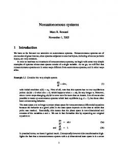
2.1.1 Single Non-Autonomous Self-Sustained Oscillator Before discussing the interactions and the respective states and phenomena (like synchronization, directionality or stability), an outline of the general characteristics of a single self-sustained oscillator subject to external non-autonomous source will be given. Consider an oscillator dx/dt = f(x(t)) with a stable periodic solution x(t) = x(t + T ) in an absence of external influence, characterized by a period T . The field f(x(t), t) can be set to be an explicit function of the time. This will be the case, for instance, if one or more of the parameters that characterize f are bounded (periodic or non-periodic) functions of time. The periodic solution x(t) is, in general, lost; and the definition of the period T becomes somewhat “blurred”. An example of such non-autonomous oscillator is presented on Fig. 2.1. In the absence of a periodic solution x(t) = x(t + T ), the definition of period could be replaced by the concept of “instantaneous period” (and correspondingly “instantaneous frequency”): at any instant of time τ the instantaneous period T (τ ) of the dynamics is the period of the limit cycle solution of f(x(t), τ ), with τ fixed. Following the definition of phase-function, given by Kuramoto [20], a generalization for non-autonomous oscillators can be discussed. In an autonomous system, the phase over the limit cycle is defined as quantity which increases by 2π during each cycle of the dynamics. A non-autonomous version of the phase-function φ(x, t) could then be defined as: dφ(x, t) ∂φ(x, t) = ω(t) + , dt ∂t
2 1
x˙ (t)
Fig. 2.1 Phase portrait of non-autonomous van der Pol oscillator with time-varying frequency. The black line is for autonomous ( A˜ = 0) and grey line for non-autonomous ( A˜ = 0.3) portrait. The system is given as: x¨ − μ(1 − x)x˙ + [ω + A˜ sin(ωt)] ˜ 2 x = 0, where ω = 1, ω˜ = 0.01 and μ = 0.2
(2.1)
0 −1 −2 −2
−1
0
x (t)
1
2
2.1 Non-Autonomous Systems
13
where ω(t) ≡ 2π/T (t) is the instantaneous frequency, i.e. the characteristic frequency of the limit cycle of the dynamics defined at a given time: �
T (τ )
ω(τ ) = 1/T (τ )
�x φ(x(t), τ ) · f(x(t), τ )dt,
0
a natural generalization of the phase for an autonomous oscillator where dφ(x)/dt ≡ 2π/T = �x φ f(x). The second term in (2.1) can be present for example due to the non-isochronoucity of the oscillator i.e. due to the effect that the perturbed amplitudes have on the phase dynamics.
2.2 Synchronization of Non-Autonomous Self-Sustained Oscillators Synchronization between coupled oscillator is a universal physical phenomenon that arises in many areas of science. It is defined as: mutual adjustment of rhythms due to weak interactions between oscillatory systems [3]. When the oscillators are weakly nonlinear and the couplings are weak as well, the synchronization phenomenon can be described qualitatively and sufficiently well by the corresponding phase dynamics. The latter is often referred to as phase synchronization [3, 11]. To set up a general description of synchronization between non-autonomous systems, two nonautonomous oscillators are set to interact through coupling function g1 , g2 parameterized by the coupling constants �1 , �2 1 : x˙ 1 =f1 (x, t) + �1 (t)g1 (x1 , x2 ) x˙ 2 =f2 (x, t) + �2 (t)g2 (x1 , x2 ). When the frequency mismatch is relatively small, one can observe for which parameter values the system is synchronized and does not exhibit phase-slips [3], i.e. when |ψ(φ1 , φ2 , t)| < constant, where the phase difference is defined as2 : ψ(φ1 , φ2 , t) ≡ φ2 (x2 (t), t) − φ1 (x1 (t), t) . Using Eq. (2.1) the time derivative of the phase difference dψ/dt can be expressed explicitly as: dψ(φ1 , φ2 , t) = (�x φ2 ) (f2 (x2 , t) + �2 g2 (x1 , x2 )) dt − (�x φ1 ) (f1 (x1 , t) + �1 g1 (x1 , x2 )) ∂φ(x2 , t) ∂φ(x1 , t) − + ∂t ∂t 1 In general, the coupling parameters and functions can also be time-dependent (as discussed later), but for simplicity and clarity they are considered autonomous in this notation. 2 The following statement holds also for higher frequency ratios in the form ψ = nφ − mφ where 2 1 n and m are integer numbers.
14
2 Theoretical Background: Non-Autonomous Systems and Synchronization
= �2 �x φ2 · g2 (x1 , x2 ) − �1 �x φ1 · g1 (x1 , x2 ) 2π 2π ∂φ(x2 , t) ∂φ(x1 , t) − + − . + ∂t ∂t T2 (t) T1 (t) The synchronization condition |ψ(φ1 , φ2 , t)| < constant will be satisfied if there exists a stable solution for the dynamics dψ(φ1 , φ2 , t)/dt. Because the velocity field i ,t) is a function of time explicitly dependant on the terms ∂φ(x , the existence of a ∂t stable equilibrium ψeq (t) satisfying dψ(φ1 , φ2 , t)/dt = 0 does not mean that the relative phase remain constant. Not even the existence of a time-dependent stable root can guarantee an absence of phase-slips: as ψeq (t) changes, the instantaneous phase difference ψ(t) may fall outside the basin of attraction, in which case a phase-slip occurs, perhaps to another equilibrium point. But if ψeq (t) changes in time slowly enough for the solution ψ(t) to remain continuously within its attracting basin, then the phase difference will vary with time (as imposed by the non-autonomous source) while the system remains within the state of synchronization.
2.3 Phase Oscillators Model When limit-cycle oscillators are coupled weakly, their interactions can be studied by means of phase oscillators [20]—which, by neglecting the amplitude dynamics, represent approximative notation of the oscillators’ full dynamics. The justification of the latter arises because the amplitudes are robustly stable, unlike the phase dynamics which correspond to the direction of the limit-cycle and are border-line stable. In terms of Lyapunov exponents this means that the amplitude dynamics are described by negative, while the phase with zero Lyapunov exponents. This sensitive stability of the phase dynamics can be easily affected even by weak perturbations in terms of coupling interactions or other external sources. Therefore, the phase oscillators serve as functional models that can describe qualitatively the interactions, the synchronization phenomenon and the corresponding transitions. A simple model of two coupled phase oscillators is used for the study of synchronization phenomenon under the influence of external non-autonomous sources. This elementary model does not capture the whole dynamics (mostly because it omits the amplitude dynamics), but serves as a good starting example where the synchronization phenomenon and the respective qualitative nature can be observed in easy and transparent way. The following also presents one of the most used procedures for treating non-autonomous problems—which includes reductions to autonomous form and multiple time scale analysis [21, 22]. The model consists of two phase oscillators, where the frequency of the first oscillator is periodically perturbed:
2.3 Phase Oscillators Model
15
dφ1 = ω1 + A˜ sin(ωt) ˜ + �1 sin(φ2 − φ1 ) dt dφ2 = ω2 + �2 sin(φ1 − φ2 ). dt
(2.2)
The two oscillators are synchronized if their phase difference is bounded |φ2 (t) − φ1 (t)| = |ψ(t)| < const [3], and if the equilibrium solution remains in its basin of attraction. Hence, for synchronization purposes the dynamics of Eq. (2.2) can be studied through the phase difference ψ(t) dynamics. The non-autonomous source (for different frequency and amplitude) can affect the dynamical behavior of the phase difference and the synchronization state itself. Instead of being constant, like in autonomous case, now the phase difference can vary with time, as imposed by the non-autonomous source. If the amplitude of the non-autonomous source is relatively large, for certain time intervals the oscillators can go in and out of synchrony—which due to the periodicity of the perturbation can result in intermittent synchronization. The effect of the non-autonomous sources on the dynamical behaviour of the interacting oscillators including amplitude dynamics, will be discussed in more detail in Sect. 2.4. The equations in system (2.2) are nonlinear non-autonomous equations that can not be solved exactly. In such situation the most common approach for analytical treatment of non-autonomous equations is introducing an additional dimension for the independent variable. Even though mathematically not fully justified (for reasons discussed above in Sect. 2.1), this procedure often allows useful analysis to be conducted. If the oscillating frequency mismatch (ω = ω2 − ω1 ) is significantly larger compared to the frequency ω˜ of the non-autonomous source (ω/ω ˜ � 1), one can try to analyze the dynamics on two separate and independent time scales (slow and fast). When the frequency ω˜ is smaller than the order of the other parameters—singular perturbation theory can be applied. Grouping the phases into the phase difference variable ψ(t) = φ2 (t) − φ1 (t) and transforming the equations to autonomous form, system (2.2) becomes: dψ = ω − A˜ sin(z) − � sin(ψ) dt dz = εν, dt
(2.3)
where ω˜ = εν, with ε being the small parameter and ν = const; and the frequency mismatch is ω = ω2 − ω1 with group coupling � = �1 + �2 . The variable ψ(t) is fast, while z(t) is slow variable. First, system (2.3) is analyzed for slow time-scale by introducing τ = εt and rescaling accordingly to:
16
2 Theoretical Background: Non-Autonomous Systems and Synchronization
(a)
(b)
(c)
ψ(t) mod 2π
6
1.2
1.2
5
1
0.8 800
4
4
2
0.8
1
0.6
0 500 1000 1500
1000
1
2 0.6
900
(d)
3
0.8
0.4
(e)
1.6
6
600
Time [s]
1000
1400
Time [s]
1800
0 670 675 680 685
Time [s]
0 20 40 60 80
Time [s]
Fig. 2.2 a–d Comparison of slow time scale analytic solution (2.5)-red line and numerical simulation of the full system (2.2)-grey line, with A˜ = 0.1, ω˜ = 0.009, ω = 0.4 and � = 0.55: (a) synchronization case, (b) intermittent case A˜ = 0.19—horizontal red line indicates where solution (2.5) is not defined: c enlarged transitions segment from (b): (d) synchronous case for fast external force ω˜ = 1. (e) The fast time scale analytic solution (2.7) with black: dashed line for synchronization case, and with full line unsynchronized case for � = 0.36 exhibiting phase slips
ε
dψ =ω − A˜ sin(z) − � sin(ψ) dτ dz =ν. dτ
(2.4)
As ε → 0 the trajectories of system (2.3) converge during slow epochs to solutions of the slow subsystem (2.4)—often called the critical manifold or quasi-steady state. Substituting τ back for the z variable (z = τ ν = ωt), ˜ the solution of the slow subsystem is expressed as: ψ(t) = arcsin
� ω − A˜ sin(ωt) ˜ � . �
(2.5)
The results, for particular parameters are presented on Fig. 2.2. The synchronized case on Fig. 2.2a shows the phase difference variations with period T = ω/2π, ˜ while the intermittent synchronization and the transitions to in and out of synchrony are presented on Fig. 2.2b. Both examples demonstrate that for slow non-autonomous source, solution (2.5) resembles the dynamics in good agreement with the numerical simulation (compare red and grey lines). The stability of the phase difference ψ(t), and thus the synchronization state, can be determined by linearization about the quasi-steady equilibrium. Linearization for the solution (2.5) yields: � dψ(t) [ω − A˜ sin(ωt)] ˜ 2 = −� 1 − . dt �2
2.3 Phase Oscillators Model
17
The stability requirement (dψ(t)/dt < 0) gives the synchronization condition: ˜ [ω− Asin( ωt)]/� ˜ < 1. The latter allows the critical couplings for transitions between synchronization, intermittent synchronization and non-synchronization to be determined: ⎧ ⎪ � > ω + A˜ : synchronization ⎨ ω − A˜ < � < ω + A˜ : intermittent synchronization ⎪ ⎩ ω − A˜ > � : non-synchronization Even though the solution for the slow time scale (2.5) qualitatively captures the dynamics (as shown on Fig. 2.2a, b), it fails to describe the fast transitions, as pointed out on the enlarged segment on Fig. 2.2c. Also the dynamics perturbed by faster nonautonomous sources can not be described by the same solution—Fig. 2.2d. This is where the fast epochs of the original system play an important role. During the fast time-scale, as ε → 0 the trajectories of system (2.3) converged to solutions of: dψ = ω − A˜ sin(ωt ˜ 0 ) − � sin(ψ), (2.6) dt ˜ 0 in the limit ε → 0. Equawhere dz(t)/dt = 0, hence z(t) = const = z 0 = ωt tion (2.6) describes autonomous case of two coupled phase oscillators—the solution of which can be express as:
� 1 1 � 2 2 2 2 t ωa − � tan ωa − � + � , ψ(t) = arctan ωa 2
(2.7)
where ωa = ω − A˜ sin(ωt ˜ 0 ) for simpler notation. The latter solution Eq. (2.7) is responsible for the dynamics of the fast synchronization transitions. The phase slips appearing where the slow-time scale solution is not defined (horizontal lines, Fig. 2.2b, c)—are govern by dynamics described by this solution (2.7)—Fig. 2.2e. The fast initial transient dynamics are also described by Eq. (2.7). The physical interpretation implies that the effect from the fast external sources on averaged is reduced within one cycle of oscillation, and the variations of ψ(t) are hinder, converging to the autonomous case. For the intermediate case when the external variation is moderately fast and not very slow, the effect on the synchronization i.e. phase difference is significantly reduced but still present. For example, if one keeps the same amplitude, but varies the speed of the non-autonomous term gradually from very slow to very fast— the variations of the phase difference will gradually decrease (and so the effect on synchronization), until the limit for very fast scale ε → 0 is reached. As described, at this point the variations of the phase difference completely vanish, and the state of the autonomous coupled systems is reached. The multiple time-scale approach allowed the dynamics of the full system (2.2) to be described and understand by analyzing the fast and slow time-scale subsystems (2.3) and (2.4), respectively. The solution (2.5) of the slow subsystem described
18
2 Theoretical Background: Non-Autonomous Systems and Synchronization
the time-varying dynamics and the intermittent synchronization transitions. The fast time-scale solution (2.7) converged to solution of autonomous synchronization case. The latter solution described the fast transitions and the phase slips dynamics during the unsynchronized states.
2.4 Limit-Cycle Oscillators Model In this section the synchronization phenomenon is presented on a model of interacting limit-cycle oscillators. The effect of the non-autonomous sources on the interactions is studied both on phase and amplitude dynamics. Dynamical characterization is also shown for different types of non-autonomous sources, acting on several important properties of the oscillators’ interaction. The systems also serve as model for determination of the stability and synchronization state.
2.4.1 The Model The Poincaré oscillator was chosen as an example of a non-autonomous limit-cycle system whose dynamical field can be made explicitly time-dependent. In polar coordinates (r, φ), it rotates at a constant-frequency, attracted with exponential velocity towards the radius, r˙ = αr (a − r ); φ˙ = ω. Here φ represents both the angle variable and the phase of the oscillator, making it isochronous oscillator. Another advantageous property of the Poincaré oscillator is that the signal is purely sinusoidal, without any high frequency harmonics, which allows better traceability of any frequency variations over time. A model of two weakly interacting Poincaré oscillators in terms of Euclidean coordinates, takes the form: x˙1 = −q1 x1 − ω1 (t)y1 + �1 (t)g11 (x1 , x2 ) y˙1 = −q1 y1 + ω1 (t)x1 + �1 (t)g12 (y1 , y2 )
(2.8)
x˙2 = −q2 x2 − ω2 (t)y2 + �2 (t)g21 (x1 , x2 ) y˙2 = −q2 y2 + ω2 (t)x2 + �2 (t)g22 (y1 , y2 )
(2.9)
qi = αi
xi2 + yi2 − ai .
The dynamics of each subsystem is described by states (xi , yi ), where i = 1, 2 denotes the oscillator. Parameters αi and ai are constants (ai being the amplitude parameter), ωi are angular frequencies, �i are the coupling amplitudes and gi1 (x1 , x2 ),
2.4 Limit-Cycle Oscillators Model
19
gi2 (y1 , y2 ) are the coupling functions. The frequency and coupling parameters each consist of a leading constant part and a small non-autonomous term: ω1 (t) = ω1 + A˜ 11 sin(ω˜ 11 t), ω2 (t) = ω2 + A˜ 21 sin(ω˜ 21 t), �1 (t) = �1 + A˜ 12 sin(ω˜ 12 t) and �2 (t) = �2 + A˜ 22 sin(ω˜ 22 t), where A˜ i1 and ω˜ i1 are small compared to ωi , while A˜ i2 and ω˜ i2 are small compared to �i . Note that, in the absence of the non-autonomous terms ( A˜ 11 = A˜ 12 = A˜ 21 = A˜ 22 = 0), the oscillators generate self-sustained oscillations [19, 23]. This implies that the non-autonomicity here should be seen, not as a source of oscillations, but more as an external perturbation/influence on the autonomous form of the oscillators, which of course have their own inherent oscillatory dynamics. In this case, the non-autonomous terms present in the system (2.8, 2.9) obviously come from periodic external modulations—some forms of non-periodic non-autonomous terms, and their implications for synchronization, are discussed in Sect. 2.4.6.
2.4.2 Analytic Calculations As already indicated, the phases of the oscillators in Eq. (2.8) are given by the angular coordinate φ: yi d arctan , φ˙ i = dt xi where the ar ctan is defined as four-quadrant operation. Developing the right-hand term for the derivative of the phase difference ψ˙ ≡ φ˙ 2 − φ˙ 1 , one obtains: cos φ2 sin φ2 ψ˙ = −ω2 (t) + ω1 (t) + �2 (t)g22 (x1 , x2 ) − �2 (t)g21 (x1 , x2 )+ r2 r2 cos φ1 sin φ1 − �1 (t)g12 (x1 , x2 ) + �1 (t)g11 (x1 , x2 ). (2.10) r1 r1 The case where the coupling functions are linear and of the form: g1 (x1 , x2 ) = x2 − x1 , g2 (y1 , y2 ) = y2 − y1 , g3 (x1 , x2 ) = x1 − x2 , g4 (y1 , y2 ) = y1 − y2 was considered. After some trivial algebra, the analytic expression for ψ˙ is obtained (details given in Appendix B). Next, a change of variables was performed by substitution of φ2 = ψ + φ1 . Because φ1 changes much faster that ψ, one can average ψ˙ by integrating over φ1 : ˙ = 1 �ψ� 2π
�
2π 0
r1 r2 ˙ sin ψ. ψ dφ1 = −ω2 (t) + ω1 (t) − �2 (t) + �1 (t) r2 r1
Similarly, after the integration of the fast variable, one can write the mean velocity of the amplitudes r1 and r2 as: 1 �˙r1 � = 2π
� 0
2π
r˙1 dφ1 = a1 r1 α1 − r1 2 α1 − �1 (t)(r1 − r2 cos ψ)
20
2 Theoretical Background: Non-Autonomous Systems and Synchronization
1 �˙r2 � = 2π
�
2π
r˙2 dφ2 = a2 r2 α2 − r2 2 α2 − �2 (t)(r2 − r1 cos ψ).
0
To obtain an equilibrium solution for the synchronization regime requires that one solves ⎧ � � ⎪ ˙ = ω1 (t) − ω2 (t) + − r2 �1 (t) − r1 �2 (t) sin ψ = 0 ⎪ ψ ⎨ r1 r2 2 α − r � (t) + r � (t) cos ψ = 0 (2.11) r ˙ = a r α − r 1 1 1 1 1 1 1 1 2 1 ⎪ ⎪ ⎩r˙ = a r α − r 2 α − r � (t) + r � (t) cos ψ = 0 2
2 2 2
2
2
2 2
1 2
and analyze the equilibrium of the system in respect of the three variables ψ, r1 , r2 . To find the solution for the system in Eq. (2.11) a numerical multidimensional minimizer [24] was employed, which returns a solution {ψeq , r1eq , r2eq }. The equilibrium is ˙ r˙1 , r˙2 }, in stable when the eigenvalues of the Jacobian matrix of the functions {ψ, respect of the three variables {ψ, r1 , r2 }, have negative real parts. It is important to note that this approach of stability analysis through the eigenvalues for the parameters at each time i.e. through instantaneous eigenvalues, is not valid in general when the systems are time-varying. There are number of practical examples, however, where this approach has been safely used for determination of synchronization [25, 26], but also some counter examples were pointed out as well [27]. For the model under investigation and the types of non-autonomous sources considered, this approach was able to determine correctly the stability of system (2.11) and the synchronization state. The last was consistent with other methods for synchronization detection, Lyapunov exponents evaluation and numerical bifurcation analysis.
2.4.3 Dynamical Behaviour and Synchronization Analysis There are many natural oscillatory systems that have characteristic frequencies which vary in time, examples being the cardiovascular system [28–30] and brain [31]. In order to understand them, one needs to consider the origins of this variability and to establish how it affects the nature of the oscillations and the mutual interactions between the oscillators. As a first step, synchronization between a pair of limit-cycle oscillators is studied, where one of the oscillators has an explicitly time dependent frequency. It is unidirectionally coupled to the other oscillator, which is autonomous. The two Poincaré oscillators (2.8) and (2.9) are set up with the following parameters: αi = ai = 1, �1 = 0, �2 = 0.38, f 1 = 1 Hz, f 2 = 0.95 Hz (where ωi = 2π f i ; i = 1, 2) and the coupling functions are specified as linear g21 (x1 , x2 ) = x1 − x2 and g22 (y1 , y2 ) = y1 − y2 . The oscillating frequency of the first oscillator is timevarying due to the presence of the non-autonomous term—in respect of parameters this mean that A˜ 11 = 0.23 and f˜11 = 0.003 Hz, and the other parameters are A˜ 12 = A˜ 21 = A˜ 22 = f˜12 = f˜21 = f˜22 = 0.
2.4 Limit-Cycle Oscillators Model
21
(a) (b)
(c)
(d)
Fig. 2.3 Dynamical behaviour of the unidirectionally-coupled (1 → 2) Poincaré oscillators (2.8, 2.9), with slow periodic variations in the frequency of oscillator-1. The parameter values used are given in the text. a Signals x1 (t) and x2 (t) are shown by the full and dashed lines respectively. Parts b and c show time-frequency analyses of x1 (t) and x2 (t) respectively using the wavelet transform. The variations in frequency and amplitude can be seen from the lines of peak values, and their projections on the amplitude-time planes, respectively. d Comparison of analytically evaluated (r2 (t), ψ(t)) and numerical (x2 (t)) analyses. The values for ψ(t) are given in {−π, π} radians
The model was simulated numerically by fourth-order Runge-Kutta integration; the same method was also used for the other simulations described below. The time evolution of the signals is shown on Fig. 2.3a. The corresponding time-frequency wavelet representation of the first oscillator is shown in Fig. 2.3b (details about wavelet analysis are given in Chap. 4). The time-frequency variations of the peak value line are clearly evident. For the chosen parameters, the oscillators can synchronize, even though the frequency of the first oscillator is time-varying. The second oscillator oscillates with a correspondingly time-varying frequency Fig. 2.3c, due to the effect of synchronization. The oscillator has turned from one whose frequency is constant into one whose frequency is time-varying, and in order to retain the phase locking its amplitude also starts to vary with time (shown in Fig. 2.3a and on the projection in Fig. 2.3c). The variations of r2 and ψ are presented in Fig. 2.3d. It is immediately evident that the phase difference is not constant (as in classical autonomous synchronization) but varies with time, as imposed by the non-autonomous term. The evaluation of the stability condition of (r1eq (t), r2eq (t), ψeq (t)) for system (2.11) showed that the two oscillators are synchronized. Next, it was investigated what happens when the two oscillators lose synchrony. The coupling was set to �2 = 0.26 and the amplitude of the non-autonomous term was increased to A˜ 11 = 0.25; (all the other parameters were same as in Fig. 2.3). It was found that for some intervals within the period of the non-autonomous modulation (the light gray regions in Fig. 2.4a) the conditions for synchronization do not hold: (r2eq (t), ψeq (t)) is unstable or does not exist, a continuously-running phase appears and the two oscillators lose synchrony. More precisely, they go in and out of synchrony as time passes, i.e. there is intermittent synchronization. The existence of synchronization and the corresponding transitions were investigated by application of method for the detection of phase synchronization—
22
2 Theoretical Background: Non-Autonomous Systems and Synchronization
(a)
(b)
(c)
Fig. 2.4 Intermittent synchronization transitions for unidirectionally coupled (1 → 2) Poincaré oscillators (2.8, 2.9). a r2 (t), ψ(t) are obtained from analytic calculations and x2 (t) (only its envelope is resolved) from numerical simulation. The light gray regions indicate the non-synchronous state. The dashed lines of ψ(t), r2 (t) within this state indicate existence of phase-slips or that an analytic solution does not exist. b 1:N synchrogram for the case under (a). c 2:N synchrogram showing synchronization transitions from 2:2 to 2:3 ratio
synchrogram [3] (Fig. 2.4b, c. Details of the implementation are given in Appendix C.) The synchrogram provides a qualitative measure where (for autonomous systems) the appearance of horizontal lines is normally taken to correspond to the synchronous state. The method clearly detect synchronization consistently with our analysis. The synchrograms show, however, that now synchronization is characterized by a smooth curve rather than a horizontal line, owing to the continuously changing phase shift induced by the non-autonomous modulation. The non-autonomous source can also induce transitions between different frequency synchronization ratios. This situation is often encountered in high order interactions of open oscillatory systems—obvious example being the cardiorespiratory system (to be discuss in later chapters). Numerical example of this kind is presented on Fig. 2.4c—the Poincaré oscillators (2.8, 2.9) now had quadratic coupling function g21 (x1 , x2 ) = (x1 − x2 )2 and g22 (y1 , y2 ) = (y1 − y2 )2 , with other parameters A˜ 11 = 0.4, ω˜ 11 = 0.008 Hz, ω1 = 2, ω2 = 3.013 and �2 = 0.8. The synchrogram shows consecutive transitions from 2:2 (or 1:1) to 2:3 frequency locking, with short non-synchronized epoches in between. The external influence caused not only the system to loose and gain synchrony, but also induced qualitative transitions between different synchronization states.
2.4 Limit-Cycle Oscillators Model
23
Another important property that defines the states of an interaction is the coupling strength. Similarly, to the previously discussed case of time-varying frequency, the coupling parameter can also be affected by non-autonomous force, turning the synchronization state time-varying. The corresponding phase difference and amplitudes will turn time-varying, while the oscillating frequencies will not vary substantially. There can be synchronization transitions depending on the nature of the external force. The definition states that the synchronization phenomenon is a result of the interplay between the frequency missmach and weak interaction between the oscillators. Hence, the interaction of oscillators found in nature often encounter the case where a non-autonomous external modulation is acting on both the frequency and the interaction strength at the same time. Moreover, the time-varying interactions can be bidirectional, affecting both of the oscillators and the underlying synchronization state. Such circumstances are relatively complex, but they reflect more closely the time-variability present in the open complex oscillatory systems found in nature [28]. Therefore, the two Poincaré oscillators were investigated each with non-autonomous time-varying frequency, interacting bidirectionally, with the coupling amplitude time-varying as well. This represents the full model (2.8, 2.9) i.e. where all the components are active and none of the parameters is zero. Furthermore, the non-autonomous parameters were considered to be unequal, so that the timevariability introduced is different in each oscillating frequency and coupling amplitude. In respect of non-autonomous parameters this meant that: A˜ 11 = 0.3, A˜ 21 = 0.225, A˜ 12 = 0.155, A˜ 22 = 0.13, f˜11 = 0.005, f˜21 = 0.0075, f˜12 = 0.004 and f˜22 = 0.0045. The rest of the parameters were set to be: αi = ai = 1, �1 = 0.32, �2 = 0.4, f 1 = 1 Hz and f 2 = 0.95 Hz. The results presented on Fig. 2.5 indicate that due to the external forces, both of the amplitudes and the frequencies are varying with time, while the oscillators are in a state of synchronization. The form of the variations is rather complex, even though the non-autonomous sources are simple periodic signals. It is important to note that this complex figure will cause potential difficulty to a data analyst when trying to identify the nature of the dynamics and the effect on synchronization. Therefore, proper tools are needed for inference and analyses of the underlaying dynamical characteristics. The external source can affect different properties of the systems, here only the cases that are of interest for this study were outlined. For example, the unidirectionally coupling can be reverse, where the autonomous can drive the non-autonomous oscillator. In this case the time-variability can be reduced or totally suppressed. The non-autonomous source can affect not only the parameters, but also the functional relationship existing among the oscillators. Very important example of this kind is the time-variability of the coupling function—for which special attention will be given in the next chapter.
24
(a)
2 Theoretical Background: Non-Autonomous Systems and Synchronization
(b)
(c)
Fig. 2.5 Numerical simulations of bidirectionally coupled Poincaré oscillators (2.8, 2.9), with variations in the oscillator frequencies and the strengths of the inter-oscillator couplings, but such that the oscillators remain in synchrony. a Signals x1 (t) and x2 (t) are indicated by full blue and grey dashed line respectively. Time-frequency wavelet analysis is applied (b) to x1 (t) and (c) to x2 (t)
2.4.4 Stability and Bifurcation Analysis This section presents the analysis needed to determine the stability of synchronization state of non-autonomous oscillators. Note that the investigating is not focused on the stability of the oscillators themselves, but on the stability of the composite system (2.11), through which one can determine whether or not the two oscillators are synchronized [3, 32]. One can do this by evaluation of the three eigenvalues obtained from the Jacobian matrix of the linearized system (2.11), λ1 , λ2 , λ3 , for given parameters at every instant of time. Because the oscillating systems (2.8, 2.9) have a relatively large number of parameters, especially those coming from the four non-autonomous terms, there are rich possibilities for dynamical changes in stability and bifurcations: e.g. changes in stability, bifurcation points, changes in the nature of stability, the existence or absence of a solution, etc. For the sake of clarity, the presentation is restricted to the case of unidirectional coupling with only one nonautonomous source applied to the oscillating frequency. The parameters of the model are the same as in the example of Fig. 2.3, except for �2 = 0.255, A˜ 11 = 0.23 and f˜11 = 0.0015 Hz. Figure 2.6a shows the signal x2 (t) from the second oscillator together with the real and imaginary parts of the corresponding eigenvalues, from which one can observe the stability of system (2.11) over a long time span. The actual stability analysis for the transition from synchronization to non-synchronization (and vice versa) will be discussed in relation to the short time segment shown in Fig. 2.6b. The stability will be investigated through observation of the eigenvalues in four characteristic regions. In region I, the real parts of the eigenvalues are all negative and there are no imaginary parts (they are all equal to zero). This means that the equilibrium solution of (2.11) is a stable node and that the two oscillators are synchronized. On crossing into region II, two complex conjugate eigenvalues appear. The real parts are still negative, however, and so the equilibrium is still stable, but it has now turned into a stable spiral. When crossing from region II into region III.1, the real parts of the complex eigenvalues become positive, and a Hopf bifurcation occurs. This point is denoted by the small circle in Fig. 2.6b. The equilibrium has become unstable and,
2.4 Limit-Cycle Oscillators Model
(a)
25
1
x (t);
0.5
Im(λ ) i
2
0 −0.5
x
Re(λ )
2
i
−1
(b)
2
x (t); ψ(t)−1;
1.2
III.2
III.1
II
I ψ
0.8
x
Im(λ ) i
2
0.4 Re(λ ) i
0 680
720
760
800
Time [s] Fig. 2.6 Stability analysis of the synchronization state for unidirectionally-coupled (1 → 2) Poincaré oscillators (2.8, 2.9). a Three black lines for the real parts of the eigenvalues of system (2.11) (with solid, dashed and dotted lines) and three brown lines for the imaginary part of the eigenvalues of system (2.11), together with signal x2 (t). Note that the lines overlap occasionally. Two different colors exist for the qualitatively distinct (real and imaginary) groups of lines. b Loss of synchronization and stability through a Hopf bifurcation together with other stability/synchronization characteristic regions: I–III.2 (separated by black vertical dashed lines). This panel provides enlarged time segment for one transition from (a); cf. the time scale on (a) compared with (b)
because the imaginary parts still exist, it is an unstable spiral. Starting from entry to region III.1 the oscillators oscillate in synchrony, even though the equilibrium of (2.11) is unstable. This discrepancy can be seen as a transitional region where the synchrony is “fading away”. The phase difference ψ(t) grows rapidly (spiraling out) until phase slips appear overtly in region III.2. Here the oscillators are not in synchronization. Similarly, one can observe a stability/synchronization analysis of the case when the oscillators make a transition from the non-synchronous to the synchronous state. The phase slips then disappear and the phase difference ψ(t) decreases, spiraling inwards. Note that the bifurcation point in Fig. 2.6b is presented in terms of time, and not in respect of parameters as normally. One may do so, because the parameters are explicitly time-dependent and are thus fully determined at every instant of
26
(a)
2 Theoretical Background: Non-Autonomous Systems and Synchronization
(b)
Fig. 2.7 Amplitude-coupling bifurcation diagram describing synchronization of the Poincaré oscillators (2.8, 2.9). a The autonomous case, illustrating stable synchronization above � A . b The nonautonomous case with time-varying frequencies, where intermittent synchronization occurs within the range 0.124 < � N A2 < 0.221. Each numerical run has random initial conditions and the first transient 1,000 s are discarded
time—which is advantageous for this kind of non-autonomous analysis, because one can observe the qualitative changes through bifurcation together with the other dynamical properties (e.g. signals, instantaneous phase, synchronization state) throughout all time. For completeness, however, an alternative representation of the bifurcation phenomena, in terms of parameters is presented. The bifurcation diagram (often referred as an orbit diagram, since it does not present the unstable objects [33]) is constructed directly from the time-series of the numerical simulation of the oscillators. This classical method was used extensively in the past to study synchronization and/or chaotic behavior [34–36]. First, the method is presented for the classical case of two autonomous oscillators. The results are used later for comparison with the nonautonomous case. For autonomous oscillators, there are no time-variations A˜ 11 = 0, the two oscillators are unidirectionally coupled, the frequencies are f 1 = 0.15 Hz, f 2 = 0.11 Hz and all the other parameters are the same as in Fig. 2.3. One can observe the time series in respect of the coupling amplitude, following a long interval for transient effects to die away. For fixed values of the coupling amplitude, one plots the points from the phase space of the second oscillator each time when the first oscillator passes through a perpendicular phase plane. The latter can be interpreted also as: points equally separated in time by the period (T1 = 1/ f 1 ) of the first oscillator. In practical terms, the model (2.8, 2.9) was simulated for specified coupling amplitudes (e.g. �2 = 0.15), and then the maxima (or zero-crossing, or other) events from the first oscillator were marked. From the times of these points, one then plots vertically (for �2 = 0.15) the points of the second oscillator. The corresponding bifurcation diagram is shown in Fig. 2.7a. One may note that, for small coupling amplitudes, the points of the second oscillator are spread widely and the two oscillators are not synchronized. The bifurcation point appears for the critical coupling amplitude � A ≈ 0.192, above which the two oscillators are synchronized;
2.4 Limit-Cycle Oscillators Model
27
this state is characterized by all points for a given coupling value coinciding in a single point, and therefore forming a smooth curve as the coupling amplitude is varied. This result was in good agreement with the outcome of the analytic investigation, for which the equilibrium solution of the system (2.11) passed from unstable to stable synchronization at the critical coupling � A ≈ 0.192. Next, a bifurcation diagram in much the same way was considered, but for the non-autonomous case. The time-varying frequency case of the two unidirectionally coupled oscillators was observed with A˜ 11 = 0.1, f˜11 = 0.0025 Hz and the other parameters as in Fig. 2.7a. In constructing the bifurcation diagram one cannot assume that the points from the first oscillator are equally separated in time, because the oscillating period is now varying due to the non-autonomous source. Instead, detection of the points as the maxima of each cycle of the first oscillator was performed. This makes the method adaptive, in a sense, because one can trace the variations in order to detect the different oscillating period in each cycle. From these time events, the points of the second oscillator are plotted in respect of the coupling amplitude �2 . The corresponding bifurcation diagram is shown in Fig. 2.7b. For small coupling amplitude (�2 � � N A1 = 0.124) the points of the second oscillator are spread widely, corresponding to the two oscillators not being synchronized. For increased values of the coupling (up to �2 � � N A2 = 0.221) the oscillators are intermittently synchronized. The transitions in and out of synchrony are due to the periodicity of the non-autonomous term, while the total time in which the oscillators are in synchrony rises as the coupling amplitude increase. For a sufficient coupling amplitude, above some critical value � N A2 ≈ 0.221, the two oscillators undergo continuous synchronization: they remain phase-locked even though their oscillatory frequencies vary with time. From Fig. 2.7b one can notice that the synchronization state is not now characterized by a very dense line, but by a bounded dense region. This results from the existence of a small and bounded phase shift.
2.4.5 Non-Autonomous Phase Shift and Lag Synchronization When two oscillators are synchronized in the classical autonomous way, the phase shift is constant. In synchronization of non-autonomous self-sustained oscillators, the phase shift is varying, because the conditions (e.g. oscillating frequencies, couplings, …) for synchronization are varying in time. In other words, the interacting state is continuously changing through different synchronization states in time, with a time-varying phase shift and amplitudes—but staying synchronized all the time, with a continuously stable solution for the phase difference (system (2.11)). The time-varying phase shift implies immediately that, under these conditions, lag synchronization [37, 38] is not possible. This was verified by the use of a similarity function S, which quantifies the time-averaged difference between the two state variable x1 , x2 taken with the time shift τ , [37]:
28
2 Theoretical Background: Non-Autonomous Systems and Synchronization
S 2 (τ ) =
�[x2 (t + τ ) − x1 (t)]2 � . [�x12 (t)��x22 (t)�]1/2
By analyzing the minimum σ = minτ (S(τ )), one can determine whether the two oscillators undergo lag synchronization. It was found that in synchronization of nonautonomous oscillators, the minimum σ cannot be sharp and nearly equal to zero (and that the minimum σ is always larger than that from autonomous synchronization under the same conditions). This is because neither the time lag nor the amplitude is constant over the whole time of observation. For very large couplings the variations of the phase difference and the amplitudes can be suppressed. The two states then became identical, x1 (t) = x2 (t), and the oscillators are in complete synchronization.
2.4.6 Sources of Non-Autonomous Dynamics The external modulations acting as sources of non-autonomicity can be of widely differing natures, forms, intensities and speeds. In the above discussion, for the sake of clarity and simplicity, the non-autonomous external source was taken to be periodic with a simple sinusoidal form. In general, of course, the external source may be of a more complex form and nature, e.g. quasi-periodic, non-periodic, chaotic, or stochastic.
2.4.6.1 Conditions The non-autonomous term itself should fulfil two conditions in order to affect the underlying onset of synchronization (or at least to do so in the manner considered in this study): 1. The amplitude of the external source should be relatively bounded with intensity smaller then the property affected. For example the A˜ 11 in Sect. 2.4.3 on Fig. 2.3 should be small compared to ω1 . For very large intensity the oscillatory dynamics may become qualitatively different (for example, exhibiting chaotic behavior or unstable oscillations), which would be beyond the scope of our interest—which is synchronization between weakly-coupled limit-cycle oscillators. 2. More important, the variations should be slow compared to the oscillatory dynamics of the affected oscillator. In other words, if the frequency of the nonautonomous term is equal to, or larger than, the frequency of the oscillators, the variations do not affect qualitatively the onset of synchronization. This was the consequence of the fast-time scale solution from the coupled phase oscillators model in Sect. 2.3. The point is that, if the non-autonomous external source introduces variations that are faster than the period of oscillation, they can be averaged within one period of the oscillations, not affecting the synchronization state.
2.4 Limit-Cycle Oscillators Model
29
Stochastic External Source Interactions between oscillators in the presence of random stochastic processes have been studied extensively in the past [3, 39, 40] and it has been shown that noise can either induce the synchronization between the oscillators or attenuate it [40–42]. Recently stochastic phase reduction for limit-cycle oscillators has been achieved for noises of different kinds [43, 44]. Such studies are typically based on a statistical approach (e.g. Fokker-Planck analysis): it is necessary to have a long time of observation (t → ∞) and the measures are statistically averaged over time. In practice, however, the time of observation is often restricted to shorter intervals, or there is a need to identify certain states in real time, and at every point of time, e.g. in biomedical measurements or communications. The main features of the earlier discussion of synchronization of non-autonomous oscillators are reconsidered briefly, but for the case when the non-autonomous external sources are stochastic rather than periodic. The Ornstein-Uhlenbeck stochastic process was used as the non-autonomous source of modulation in the model (2.8, 2.9): √ 2D 1 ξ(t) η(t) ˙ = − η(t) + τ τ where τ and D are the correlation time and noise strength respectively, and ξ(t) is Gaussian white noise. The statistical properties of the colored noise are then: �η(t)� ˙ = 0 and �η(t)η(s)� ˙ = Dτ e−|t−s|/τ . One can consider the unidirectionally coupled case of time-varying frequency from Sect. 2.4.3 presented on Fig. 2.3 (the same effect can be observed for time-varying couplings). The noisy source was added to the natural frequency of the first oscillator: ω1 (t) = ω1 + η(t), but all the other parameters and conditions were kept the same. The correlation time and the strength of the colored noise were τ = 50 and D = 25. The resultant numerical signal is presented in Fig. 2.8a. From Fig. 2.8b, c, it is clear that the amplitude and frequency of the second oscillator now vary too, due to the effect of the synchronization. One can noticed that, in accord with the above discussion of the frequency of variation of the non-autonomous source, only the lower-frequency components of the Ornstein-Uhlenbeck process affect the variations, whereas the higher frequencies did not, because they were faster than a period of the first oscillator. Using the observations made in Sect. 2.4.2 one can find that all the eigenvalues have negative real parts, demonstrating that the two oscillators remained synchronized while their frequencies are varying, following the dynamics of the stochastic source.
Chaotic External Source The next case to be consider was when the source of non-autonomicity is a quasi-periodic signal generated by a chaotic deterministic system. Its worth noting en passant that chaotic systems have played an important role in synchronization
30
2 Theoretical Background: Non-Autonomous Systems and Synchronization
(a)
(b)
(d)
(c)
(e)
Fig. 2.8 Synchronization of unidirectionally-coupled (1 → 2) Poincaré oscillators (2.8, 2.9), under conditions where there are stochastic (a)–(c) and quasi-periodic variations (d)–(e) in the frequency of oscillator-1. a Time evolution of the colored noise signal η(t). b The signal x2 (t) and the numerically evaluated phase difference ψ(t). c Contour plot of wavelet analysis of the signal x2 (t) from the second oscillator. d Time evolution of the chaotic signal z(t) and the signal x2 (t) from the second oscillator (seen as its envelope). e Wavelet analysis of x2 (t) from the second oscillator. The frequency variations are indicated by the black line plotting the locus of the peak values
theory, both in studying the interactions among chaotic systems and defining new synchronization concepts [7, 10, 11]. Synchronization of chaotic systems and periodic non-autonomous sources has been studied in [45, 46]. Here, the interest is more in using the non-periodic forms of signals generated by chaotic systems, rather than in the chaotic properties of the systems. The well-known Lorenz system [47] was used, in the following form: γ x˙ = σ(y − x) γ y˙ = x(ρ − z) − y γ z˙ = x y − βz
(2.12)
where the parameters were set to be: σ = 10, β = 8/3 and ρ = 28. The constant parameter γ = 0.005 was introduced in order to reduce the velocity in the system, so that the frequency of the signals would be low compared to those of the oscillators. Again the unidirectionally coupled case of synchronization was considered, with the frequency of the first oscillator being time-varying (Sect. 2.4.3, Fig. 2.3). The non-autonomous source now is taken to be z(t) from (2.12), presented in Fig. 2.8d. ˜ − c), ˜ where A˜ = The time-varying frequency is defined as: ω1 (t) = ω1 + A(z(t) 1/60, c˜ = 23 and the other parameters are all as discussed before. Under these conditions, the two oscillators can synchronize. In order for the second oscillator to be synchronized and to stay in frequency entrainment, its amplitude and oscillating
2.4 Limit-Cycle Oscillators Model
31
frequency start to vary, as imposed by the quasi-periodic non-autonomous source as shown in Fig. 2.8d, e.
2.4.7 Generalization of the Model It is reasonable to wonder to what extent the above results are general, rather than confined to the particular model (2.8, 2.9) of two Poincaré oscillators. The Poincaré oscillator as a unit, in its uncoupled form, is a radial isochronal oscillator. All trajectories starting at one point of φ go to the same asymptotic phase and, as mentioned above, the variable φ represents both the phase and the angle variable (φ˙ = ω). There is, however, a vast group of limit-cycle oscillators where the local oscillatory frequency depends on the local amplitude. The terms introducing this nonisochronicity are related to the shear of the phase flow near the limit cycle. Synchronization of oscillators with shear terms has been studied along with the oscillation death (BarEli) effect [32, 48]. It was reported [49, 50] that nonisochronicity can be a cause of anomalous phase synchronization in a population of non-identical oscillators. The phenomenon of synchronization between non-autonomous oscillators was observed in a variety of limit-cycle oscillators, including van der Pol and StuartLandau oscillators, as well as the Poincaré oscillators with shear terms. It was found that the qualitative characteristic of the synchronization under such non-autonomous conditions was valid for the other types of limit-cycle oscillators. The results of analogue experiments exploring synchronization between non-autonomous van der Pol oscillators will be presented in Chap. 5.
2.5 Non-Autonomous Coupling Function So far the discussion was focused on non-autonomous parameters and how they affect the interactions. Another important property that characterizes the interactions among oscillators is the coupling function. Opposite to closed autonomous oscillators, the coupling function in open oscillatory systems can vary in time, both in intensity and form. In fact, a functional relationships that characterize the cardiorespiratory interactions are time-varying (as will be demonstrated in the following chapter). But, why is coupling function important and how does it affect the interactions? It defines the functional law about the interactions and the law by which the interaction undergo transitions to synchronization i.e. transitions to equilibrium stability. (Qualitative description about the role of coupling function in oscillatory interaction is discussed in more details in Chap. 3 Sect. 3.3.2). In order to investigate how the coupling function can affect the interacting systems and cause transitions to synchronization, a special case was considered where: the time-variability of the form of the coupling function alone is the cause for synchronization transitions. This was accomplished by maintaining the parameters
32
2 Theoretical Background: Non-Autonomous Systems and Synchronization
(b) ψ (t)
(a) 2
0 −10 −20 −30
(c)
0
q 1(ψ(t))
q(ψ)
1
−1 −2 −π
0
ψ
π
2 0 −2 0
400
800
1200
1600
2000
Time [s]
Fig. 2.9 Coupling function and synchronization transition as a result of its time-variability. a Form of the coupling function Eq. (2.13) with constant a(t) = 1 and b(t) = 1. Phase difference (b) and coupling function q1 (ψ(t)) (c) for system (2.14) indicating the synchronization transition due to the variability of the function of interactions. The parameters for the coupling function are varied linearly in time: a(t) = 0 → 1.4 and b(t) = 1.4 → 0; rest of parameters are constant: �1 = 0.013, �2 = 0.01, ω1 = 0.11 and ω2 = 0.07
(frequencies ωi and coupling strengths �i ) constant, while the form of the coupling function is varying by some predefined non-autonomous source. A coupling function represented in the reduced phase model: φ˙ i = ωi + �i q(φi , φ j ), should be a 2π-periodic function. In his phase models Kuramoto [20] used a simple sine form function of the phase difference q(φ1 , φ2 ) = sin(φ2 − φ1 ), Winfree [51] used function that is defined by both phases rather than just the phase difference q(φ1 , φ2 ) = [1 + cos(φ2 )] sin(φ1 ), while Daido and Crawford [52–54] used more general form where the function can be expanded in Fourier series. Here the discussion is concentrated on numerical simulation of two coupled phase oscillators (similar to those presented with Eq. 2.2), but the coupling function for the phase difference consists of four Fourier components up to the second order: q(φ) = a(t) sin(φ) + b(t) cos(φ) + a(t) sin(2φ) + b(t) cos(2φ),
(2.13)
where the a(t) and b(t) parameters are considered to be time dependent terms. The form of the coupling function is presented on Fig. 2.9a. The simple model for investigation will then have the following form: φ˙1 =ω1 + �1 q1 (φ2 − φ1 ) φ˙2 =ω2 + �2 q2 (φ1 − φ2 ).
(2.14)
By changing the parameters a and b in time one can vary the form of the coupling function. For the case under study, the goal was to maintain the coupling strength constant while only the form of the function to vary. The latter means that besides the coupling parameters �i , also the norm of the coupling function should be constant
2.5 Non-Autonomous Coupling Function
33
throughout the time. Therefore the function parameters a and b were non-autonomous sources varying linearly (and then square rooted) in time, while the norm of the function was constant in every instant of the time. Figure 2.9b shows the phase difference ψ(t) = φ2 (t) − φ1 (t) which serves as indicator for synchronization of systems (2.14), i.e. if the phase difference is bounded (ψ < const) or not. Figure 2.9c shows the dynamical time-evolution of the coupling function (of second to first oscillator) as a function of phase difference. The two figures demonstrate that: at the beginning the oscillators are not synchronized and as the form of the coupling function is varied, the oscillators get more coherent and around time = 1000 s there is transition to full synchronization. The latter means that the coupling function changed qualitatively the dynamical behaviour, equilibrium solution appeared and synchronized stable state is reached. The non-autonomous coupling functional relation is important because it resembles the dynamics of many real oscillatory systems found in nature. One of the main systems of interest for this study, the cardiorespiratory system has coupling function which is evidently time-varying. The latter was discovered by the use of the method presented in the following chapter.
References 1. W. Horsthemke, R. Lefever, Noise Induced Transitions (Springer, Berlin, 1984) 2. A. Stefanovska, H. Haken, P.V.E. McClintock, M. Hožiˇc, F. Bajrovi´c, S. Ribariˇc, Reversible transitions between synchronization states of the cardiorespiratory system. Phys. Rev. Lett. 85, 4831–4834 (2000) 3. A. Pikovsky, M. Rosenblum, J. Kurths, Synchronization—A Universal Concept in Nonlinear Sciences (Cambridge University Press, Cambridge, 2001) 4. S.H. Strogatz, D.M. Abrams, A. McRobie, B. Eckhardt, E. Ott, Crowd synchrony on the millennium bridge. Nature 438(7064), 43–44 (2005) 5. G.B. Ermentrout, J. Rinzel, Beyond a pacemaker’s entrainment limit—phase walk-through. Am. J. Physiol. 246(1), R102–R106 (1984) 6. C. Schäfer, M.G. Rosenblum, J. Kurths, H.H. Abel, Heartbeat synchronised with ventilation. Nature 392(6673), 239–240 (1998) 7. L. Kocarev, U. Parlitz, General approach for chaotic synchronization with applications to communication. Phys. Rev. Lett. 74(25), 5028–5031 (1995) 8. B. Blasius, A. Huppert, L. Stone, Complex dynamics and phase synchronization in spatially extended ecological systems. Nature 399(6734), 354–359 (1999) 9. A.A. Castrejón-Pita, P.L. Read, Synchronization in a pair of thermally coupled rotating baroclinic annuli: understanding atmospheric teleconnections in the laboratory. Phys. Rev. Lett. 104, 204501 (2010) 10. L.M. Pecora, T.L. Carroll, Synchronization in chaotic systems. Phys. Rev. Lett. 64(8), 821–824 (1990) 11. M.G. Rosenblum, A.S. Pikovsky, J. Kurths, Phase synchronization of chaotic oscillators. Phys. Rev. Lett. 76(11), 1804–1807 (1996) 12. L. Kocarev, U. Parlitz, Generalized synchronization, predictability, and equivalence of unidirectionally coupled dynamical systems. Phys. Rev. Lett. 76(11), 1816–1819 (1996) 13. R.L. Stratonovich, Topics in the Theory of Random Noise: General Theory of Random Processes, Nonlinear Transformations of Signals and Noise (Gordon and Breach, Mathematics and its applications, 1963)
34
2 Theoretical Background: Non-Autonomous Systems and Synchronization
14. P.E. Kloeden, M. Rasmussen, Nonautonomous Dynamical Systems (AMS Mathematical Surveys and Monographs, New York, 2011) 15. M. Rasmussen, Attractivity and Bifurcation for Nonautonomous Dynamical Systems (Springer, Berlin, 2007) 16. P.E. Kloeden, Nonautonomous attractors of switching systems. Dyn. Syst. 21(2), 209–230 (2006) 17. P.E. Kloeden, Synchronization of nonautonomous dynamical systems. Elect. J. Diff. Eqns. 1, 1–10 (2003) 18. P.E. Kloeden, R. Pavani, Dissipative synchronization of nonautonomous and random systems. GAMM-Mitt. 32(1), 80–92 (2009) 19. V. Anishchenko, T. Vadivasova, G. Strelkova, Stochastic self-sustained oscillations of nonautonomous systems. Eur. Phys. J. (Special Topics) 187, 109–125 (2010) 20. Y. Kuramoto, Chemical Oscillations, Waves, and Turbulence (Springer-Verlag, Berlin, 1984) 21. M. Desroches, J. Guckenheimer, B. Krauskopf, C. Kuehn, H. Osinga, M. Wechselberger, Mixed-Mode Oscillations with Multiple Time Scales. SIAM Review 54(2), 211–288 (2012). doi:10.1137/100791233 22. B. Ermentrout, M. Wechselberger, Canards, clusters, and synchronization in a weakly coupled interneuron model. SIAM J. Appl. Dyn. Syst. 8, 253–278 (2009) 23. A.A. Andronov, A.A. Vitt, S.H. Khaikin, The Theory of Oscillators (Dover Publications Inc., New York, 2009) 24. M. Galassi, J. Davies, J. Theiler, B. Gough, G. Jungman, P. Alken, M. Booth, F. Rossi, GNU Scientific Library Reference Manual Version 1.14, Chapter 35: Multidimensional Root-Finding. (Network Theory, Bristol, 2010) 25. G.A. Johnson, D.J. Mar, T.L. Carroll, L.M. Pecora, Synchronization and imposed bifurcations in the presence of large parameter mismatch. Phys. Rev. Lett. 80, 3956–3959 (1998) 26. J.N. Blakely, D.J. Gauthier, G. Johnson, T.L. Carroll, L.M. Pecora, Experimental investigation of high-quality synchronization of coupled oscillators. Chaos 10, 738–744 (2000) 27. N.J. Corron, Loss of synchronization in coupled oscillators with ubiquitous local stability. Phys. Rev. E 63, 055203 (2001) 28. A. Stefanovska, M. Braˇciˇc, Physics of the human cardiovascular system. Contemp. Phys. 40, 31–55 (1999) 29. Y. Shiogai, A. Stefanovska, P.V.E. McClintock, Nonlinear dynamics of cardiovascular ageing. Phys. Rep. 488, 51–110 (2010) 30. J. Jamšek, M. Paluš, A. Stefanovska, Detecting couplings between interacting oscillators with time-varying basic frequencies: Instantaneous wavelet bispectrum and information theoretic approach. Phys. Rev. E 81, 036207 (2010) 31. D. Rudrauf, A. Douiri, C. Kovach, J.P. Lachaux, D. Cosmelli, M. Chavez, C. Adam, B. Renault, J. Martinerie, M.L. Van Quyen, Frequency flows and the time-frequency dynamics of multivariate phase synchronization in brain signals. Neuroimage 31(1), 209–227 (2006) 32. D.G. Aronson, G.B. Ermentrout, N. Kopell, Amplitude response of coupled oscillators. Physica D 41(3), 403–449 (1990) 33. S.H. Strogatz, Nonlinear Dyn. Chaos (Westview Press, Boulder, 2001) 34. U. Parlitz, W. Lauterborn, Period-doubling cascades and devil’s staircases of the driven Van der Pol oscillator. Phys. Rev. A 36(3), 1428–1434 (1987) 35. R. Mettin, U. Parlitz, W. Lauterborn, Bifurcation structure of the driven van der Pol oscillator. Int. J. Bifurcat. & Chaos 3(6), 1529–1555 (1993) 36. U.E. Vincent, A. Kenfack, Synchronization and bifurcation structures in coupled periodically forced non-identical duffing oscillators. Phys. Scr. 77(4), 045005 (2008) 37. M.G. Rosenblum, A.S. Pikovsky, J. Kurths, From phase to lag synchronization in coupled chaotic oscillators. Phys. Rev. Lett. 78(22), 4193–4196 (1997) 38. S. Boccaletti, J. Kurths, G. Osipov, D.L. Valladares, C.S. Zhou, The synchronization of chaotic systems. Phys. Rep. 366(1–2), 1–101 (2002) 39. B. Lindner, J. Garcia-Ojalvo, A. Neiman, L. Schimansky-Geier, Effects of noise in excitable systems. Phys. Rep. 392(6), 321–424 (2004)
References
35
40. D. Garcia-Alvarez, A. Bahraminasab, A. Stefanovska, P.V.E. McClintock, Competition between noise and coupling in the induction of synchronisation. EPL 88(3), 30005 (2009) 41. A. Neiman, L. Schimansky-Geier, A. Cornell-Bell, F. Moss, Noise-enhanced phase synchronization in excitable media. Phys. Rev. Lett. 83(23), 4896–4899 (1999) 42. J. Teramae, D. Tanaka, Robustness of the noise-induced phase synchronization in a general class of limit cycle oscillators. Phys. Rev. Lett. 93(20), 204103 (2004) 43. J.N. Teramae, H. Nakao, G.B. Ermentrout, Stochastic phase reduction for a general class of noisy limit cycle oscillators. Phys. Rev. Lett. 102(19), 194102 (2009) 44. D.S. Goldobin, J.N. Teramae, H. Nakao, G.B. Ermentrout, Dynamics of limit-cycle oscillators subject to general noise. Phys. Rev. Lett. 105(15), 154101 (2010) 45. T.L. Carroll, L.M. Pecora, Synchronizing nonautonomous chaotic circuits. IEEE Trans. Circ. Syst. II 40(10), 646–650 (1993) 46. I. Bove, S. Boccaletti, J. Bragard, J. Kurths, H. Mancini, Frequency entrainment of nonautonomous chaotic oscillators. Phys. Rev. E 69(1), 016208 (2004) 47. E.N. Lorenz, Deterministic non-periodic flow. J. Atmos. Sci. 20(2), 130–141 (1963) 48. J.J. Suárez-Vargas, J.A. González, A. Stefanovska, P.V.E. McClintock, Diverse routes to oscillation death in a coupled-oscillator system. EPL 85(3), 38008 (2009) 49. B. Blasius, E. Montbrio, J. Kurths, Anomalous phase synchronization in populations of nonidentical oscillators. Phys. Rev. E 67(3), 035204 (2003) 50. E. Montbrio, B. Blasius, Using nonisochronicity to control synchronization in ensembles of nonidentical oscillators. Chaos 13(1), 291–308 (2003) 51. A.T. Winfree, Biological rhythms and the behavior of populations of coupled oscillators. J. Theor. Biol. 16, 15 (1967) 52. H. Daido, Onset of cooperative entrainment in limit-cycle oscillators with uniform all-to-all interactions: bifurcation of the order function. Physica D 91, 24–66 (1996) 53. H. Daido, Multibranch entrainment and scaling in large populations of coupled oscillators. Phys. Rev. Lett. 77, 1406–1409 (1996) 54. J.D. Crawford, Scaling and singularities in the entrainment of globally coupled oscillators. Phys. Rev. Lett. 74, 4341–4344 (1995)
http://www.springer.com/978-3-319-00752-6