Theory and Numerical Calculations for Radially ... - IEEE Xplore

419

IEEE TRANSACTIONS ON MICROWAVE THEORY AND TECHNIQUES, VOL. 44, NO. 3, MARCH 1996

Theory and Numerical Calculations for Radially Inhomogeneous Circular Ferrite Circulators Clifford M. Krowne, Senior Member, ZEEE, and Robert E. Neidert, Member, IEEE

Abstract-This paper presents a new theory for the operation of microstrip and stripline circulators, specially set up to permit radial variation of all the magnetic parameters. A computer code, taking only a few seconds per calculated point on a modest computer, was developed from the theory, and calculated results are given. In the theory we develop a two-dimensional (2-D) recursive Green’s function G suitable for determining the electric field E= anywhere within a microstrip or stripline Circulator. The recursive nature of G is a reflection of the inhomogeneous region being broken up into one inner disk containing a singularity and N annuli. G has the correct properties to allow matching to the external ports, thereby enabling +parameters to be found for a three-port ferrite circulator. Because of the general nature of the problem construction, the ports may be located at arbitrary azimuthal angle @ and possess arbitrary line widths. Inhomogeneities may occur in the applied magnetic field Ha,,, , magnetization 4.irM,, and demagnetization factor N d . All magnetic inhomogeneity effects can be put into the frequency dependent tensor elements of the anisotropic permeability tensor. Numerical results are presented for the simpler but immensely practical case of symmetrically disposed ports of equal widths taking into account these radial inhomogeneities. Studies of breaking up the area into 1,2, and 5 annuli are undertaken to treat specific inhomogeneous problems. The computer code which evaluates the recursive Green’s function is very efficient and has no convergence problems.

I. INTRODUCTION

T

HE ferrite community has long needed a simple but accurate way to calculate circulator performance in the presence of radial variation of bias field, ferrite material type, and demagnetizing factor. Full analysis with finite element or finite difference methods is so slow, user-unfriendly, and expensive that generally useful answers about the affects of radial variations have not been forthcoming. The paper here provides a means to get these answers, at the rate of a few seconds per calculation point, with a computer code developed from a new partial mode matching theory. Previous work in the area of multiport circulators has focused on the treatment of high-symmetry geometric configurations, a limited number of symmetrically disposed ports, and a homogeneous nonreciprocating medium [I I-[ 151. The theoretical techniques for modeling the circulator have ranged from Green’s functions, boundary element methods, boundary contour integral methods, to finite element methods. Each method has special advantages and disadvantages in relation Manuscript received April 9, 1995; revised November 27, 1995. The authors are with the Microwave Technology Branch, Electronics Science & Technology Division, Naval Research Laboratory, Washington, DC 20375-5347 USA. Publisher Item Identifier S 0018-9480(96)01545-1.

to the other methods, depending upon what the researcher is interested in emphasizing in the problem. Discussion of these numerical techniques as well as other information on circulators and anisotropic media may be found in recent surveys [16], [17]. Our interest is in obtaining a formulation which allows us to inspect the physics and electromagnetics of the solution, and which can be related to earlier simple results on homogeneous problems. We also want a solution which is numerically efficient to evaluate. With these considerations, an analytical approach was taken to derive a Green’s function which would allow the circulator region to be divided up into an arbitrary number of rings of definite radial thickness. The idea was to make the rings or annuli thin enough to accurately describe the actual arbitrary radial variation of the various inhomogeneities contributing to the permeability tensor. In Sections I1 and I11 we develop a two-dimensional (2D) recursive Green’s function G suitable for determining the electric field E, anywhere within the circulator. The recursive nature of G is a reflection of the inhomogeneous region being broken up into one inner disk, containing a singularity, and N annuli. G has the correct properties to allow matching to the external ports, thereby enabling s-parameters to be found for a three-port ferrite circulator. Because of the general nature of the problem construction, the ports may be located at arbitrary azimuthal angle 4%and possess arbitrary line widths w,for the ith port. The line widths may be also measured in terms of the angular spread Acj%on the outer edge of the circular disk of radius R. Inhomogeneities occur in the applied magnetic field Happ,magnetization 47r Ms, and demagnetization factor Nd. All magnetic inhomogeneity effects can be put into the frequency dependent tensor elements of the anisotropic permeability tensor. The process of how this can be done will be discussed in Section V. Section VI gives some calculated results for a few arbitrarily selected cases of radially nonuniform demagnetizing factor, applied bias field, and ferrite material types. These calculations are for the immensely practical case of symmetrically disposed ports of equal widths. Studies of breaking up the area into l , 2 , and 5 annuli are undertaken to display the approximation levels required to treat inhomogeneous problems. The computer code, which evaluates the recursive Green’s function, is very efficient and calculation time is presented. 11. THEORY

The Green’s function to be developed below, although of a recursive nature, may in the limit be shown to reduce to

0018-9480/96$05.00 0 1996 IEEE

420

IEEE TRANSACTIONS ON MICROWAVE THEORY AND TECHNIQUES, VOL. 44, NO. 3, MARCH 1996

$I

It is the Green’s function G E H ( r , 4;R, 4’)at T = R which we are particularly interested in obtaining in this paper so that the s-parameters may be found for the three-port inhomogeneous circulator. The recursion process to be employed here is like that utilized for planar structures [23]. Maxwell’s sourceless curl equations are, for harmonic conditions with phasor time dependence exp(i w t ) assumed

=11

ISOLATED

II I

I

aWTm COMPUTATIONAL

V x E = -iwB D x H = iwD. I

$I = -lIn

!

INPUT

These two equations are valid within the ferrite disk region which is considered to be inhomogeneously loaded with material (the disk could also be a magnetically biased semiconductor region displaying the magnetoplasma effect). The constitutive relationships are given generally by

$I = +xi3 OUTPUT

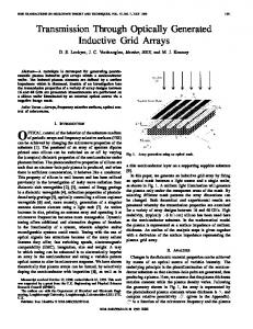
Fig. 1. Top view of a radially inhomogeneous circulator showing the inner disk labeled with index number z = 0 and the annuli indexed from z = 1 onward. Here four annuli are shown. The figure shows the special case of symmetrically disposed ports located at 4 = - x / 3 (input), x / 3 (output), and x (isolated). Angular port width is A&. A side view is shown also for a real physical circulator. Biased ferrite material of thickness H exists only for T 5 R.

either the single circular disk case [18], [19] or a circular ring [20]-[22]. We develop the Green’s function as a response to a forcing function which represents a driving function, or source function, of magnetic field type, H+s,located on the azimuthal boundary of a circular contour of radius R. Fig. 1 shows the general geometric configuration of the circulator. The forcing function has the property of limiting the field to finite values only at radius r = R and azimuthal angle locations q5 = d,, where z represents specific points along the enclosing circulator contour. The linear system of partial differential equations (PDE’s), through which H4s(r = R, q5 = 4,) imposes its forcing behavior, may be written formally in terms of one governing PDE with operator L acting on our prime field quantity of interest here, E,

LE,(r,

4) = H @ s ( R4%). ,

(1)

From E,, the other field components, H+ and H,, can be determined in this 2-D problem. Let us identify the magnetic field at location r = R to be the contour field associated with the surface in the 2-D problem we are treating

H+c(R,4s) = H d R , 4 )

(2)

where an explicit subscript is added to denote this association. H+c may be related to the physical forcing magnetic field H4s by the relation b(.

-

R ) H @ c ( R$1, = H+s(R,4).

(5) (6)

(3)

Using the properties of the Dirac delta function in the spatial radial direction and the azimuthal angular direction, we find

B=bH D = E“E.

(7) (8)

In the ferrite disk region, we will assume that the dielectric tensor reduces to a scalar E

(9)

= E.

Of course, this would not be the case for a semiconductor where we would retain the tensor permittivity and drop the tensor permeability [24], [25]. The general expression in matrix notation for the curl of an arbitrary vector field in cylindrical coordinates is

r$ VxA=

r

a+

2 8,

A, .A+ Az

1

(10)

where it is noted that the expansion of (10) is accomplished by keeping the unit vector terms outside of the partial operators d,; i = r,q5,z. It is also noted that we use r instead of the usual p for the cylindrical radius. For the 2-D problem we are constructing, it is sufficient to drop a dimension by setting

a

- = 0.

az To be somewhat consistent with notation in the circulator literature [lS], we set the permeability tensor

421

KROWNE AND NEIDERT: THEORY AND NUMERICAL CALCULATIONS FOR RADIALLY INHOMOGENEOUS CIRCULATORS

Bessel function type, and ring index)

The governing Helmholtz equation for this problem is

+

V 2 E , k&E, = 0 with the definitions k& = W2&Peff n

Pcff

= -.

-

(17)

C T41 h a l ( T )=

nri 1 ct k f f , z J A ( k f f , z~ )^-Jn(kefi,%i)]. P2

n

&A

I*

(18)

Using definition (18) in (14) and (15) provides more compact expressions for H4 and H ,

(26)

T

In these three definition equations, the general disk or annulus location index z has been used as the last index on the C,,,, and Cnhaz,on the material tensor element parameters pt and K ~ and , on the effective propagation constant Iceff,, and permeability p , ~ , For ~ . the inner disk, the index in (24)-(26) is merely i = 0, allowing us to rewrite (22) and (23) as

(19)

03

(27)

A. E, and H+ Fields in the Inner Disk The inhomogeneous circular surface is broken up into one inner disk centered at r = 0, and N annuli, each annulus labeled by index i. To be consistent in labeling notation, the inner disk is labeled with i = 0. The disk, and each annulus region is sourceless, so that the homogeneous Helmholtz equation (16) holds. The solution to (16) in cylindrical coordinates is well known to be Bessel functions multiplied by azimuthal circular harmonics. For the problem at hand, azimuthal symmetry exists, requiring that the separable circular harmonics be of type {exp(in4)}, for any integer n. Helmholtz equation (16) will therefore yield Bessel functions of integer order. Because the inner disk contains the point T = 0, the only Bessel function to be well behaved, not possessing a singularity, will be the Bessel function of the first kind, J,. Therefore the total electric field E,o in the disk must be a superposition-of

B. Fields in the Annuli Because an annulus does not include the origin, a superposition of any two linearly independent Bessel functions will be required to construct the radial part of the separable solution to (16). The electric field is therefore 03

+

E,, =

[anzJn(krff,r~) b n t N n ( k e ~ , t r ) l e l n d ; n=-cc

i = 1 , 2 , . .., N .

(29)

As in (24), let us define C n r b t ( ~ ) Nn(keff,tr) (30) so that (29) can be rewritten in the more abbreviated and transparent form 00

+

E,, =

[ a n z C l z e a z ( bnzCnebz(~)leZn4; ~) n=--00

z = 1 , 2,..., N .

giving

(31)

For the H+%field component, referring to (19) 00

Ea0

03

Em0

= n=-m 00

n=-m 00

Likewise for the magnetic fields, invoking (19) 03

Using the coefficient definition in (26) for the ani factor and the additional definition

To standardize the notation, abbreviate, and make transparent what is happening in the recursion process itself, a few definitions are made (the upper index on C is the component, and the lower indices are azimuthal mode number, field type,

H4i can be expressed in the much more compact form

IEEE TRANSACTIONS ON MICROWAVETWORY AND TECHNIQUES, VOL. 44, NO 3, MARCH 1996

422

C. Boundary Conditions and the Disk-First Annulus Intedace

harmonic

There are three distinct types of boundary condition interfaces. The first boundary condition type is at the disk-first annulus interface. This interface must match the inner disk, which contains a potential singularity at r = 0 which has been specially excluded, to the first annulus which contains two linearly independent Bessel functions out of which the E, field is constructed. Once the matching has been completed at this first interface, the field information can be pulled through to the next interface, and the matching procedure repeated. Thus, each internal interface due to two adjacent annuli involves the same matching process. These internal interfaces constitute the second type of boundary condition. If there are N annuli, then there will be exactly N, = N - 1 interfaces of the second type. The third type of boundary condition occurs at the interface between the last annulus, the a = N annulus, and the external part of the circulator geometry. This is where the last annulus or ring abuts or touches either an ideally imposed magnetic wall, which approximately expresses the transition between the ferrite material and the outside dielectric (air or a surrounding dielectric), or the transition ports taking energy into or out of the circulator. For a three-port circulator, these ports are referred to as the input port, the output port, and the isolated port. Normal practical design strategy attempts to minimize the exiting signal from the isolated port and maximize the exiting signal from the output port. There will be a total of N, 2 interfacial boundary conditions, all of the internal ones plus one disk-annulus interface and one Nth annulus-outside interface. The inner disk has radius T O . Each annulus has radius r, measured from its center. The width of each annulus is Ar, = r,o - r,I, where the subscript “0” or “I” indicates outer or inner radius of the zth annulus. It is sufficient to apply boundary constraints on either the (&, D n ) normal pair or the ( E t ,H t ) tangential pair. We choose the second pair as it is easily applied. For the first type of interfacial boundary condition

(39a) (39b) %OC&aOD - a7LlcnhalD + bnlC:hblD’ Here the argument information of the C coefficients has been compressed into a single added subscript index D which denotes radial evaluation at the disk radius D = rO = r 1 I . Solution of (39) yields for the 1st annulus field coefficients a n 1 and bnl anOCneaOD

4

aril

= anlCnealD

-

=

bnl =

+ bnlCneblD

@

CneaOD

CneblD

CnhaOD

CnhblD

CnealD

CneblD

CnhalD

CnhblD

CnealD

CneaOD

CnhalD

CnhaOD

CnealD

CneblD

CnhalD

CnhblD

These expressions may be considerably abbreviated by defining the disk-to-annulus coupling numerator factors

and the determinant D; providing the information in the ith annulus

+

G o ( r = T o ) = & l ( r = TIT) H4O(r = T O ) = H+l(r = ~ 1 1 ) .

(35)

(36)

In (42), subscript combination iA denotes a radial evaluation at the ith annulus inner radius r z I , that is TzA

= r,I = r,

Thus, we may now write

an1

-

Ar,/2.

(43)

and bnl as

D. Intra-Annuli Boundary Conditions

The ( E t ,H,) tangential pair is used to match between two adjacent annuli. Following forms (35) and (36)

Using (27) and (31) for the E, constraint, (35) becomes %z(r

00

= rzo) = &(z+l)(T

= r(z+l)I)

H4z(r = rzo) = K $ ( Z + l ) ( T = r ( z + l ) I ) .

anOCneaO(TO)eZn4

(45)

(46)

n=--00

00

=

[anlCneal(r11)

+ b n l c n e b l ( w ) l e z n @ .(37)

Invoking the annuli E, field expression in (31), and inserting it into (45)

n=-00

Utilizing (28) and (34) for the H+ constraint, (36) becomes w

anzCneaz(Tz0) -

+ bnzCnebz(Tz0)

an(z+l) C n e a ( z + l ) ( r ( z + l ) I )

+ bn(,+l)Cneb(z+l) ( r ( z + l ) I ) . (47)

n=-w 00

=

[uT%lC 4n h n l ( r l I )

+ b 7 L l C $ & 1 ( r l I ) ] eZn? (38)

n=-w

By the orthogonality of the azimuthal harmonics on ( - T , T ) , these equations may be written down for each individual nth

Similarly, for 234 recalling (34), and inserting into (46) anZCzhaz

(rZo)-k bnZC$& ( T d )

+

- a n ( z + l ) C ~4~ h a ( z + l ) ( r ( Z + l ) I ) bn(Z+l)cthb(z+l) (‘(Z+l)I).

(48)

423

KROWNE AND NEIDERT: THEORY AND NUMERICAL CALCULATIONS FOR RADIALLY INHOMOGENEOUS CIRCULATORS

These two equations may be compressed by defining the fifth index on the C coefficients to be the outer radius T ~ Oof the ith annulus or the inner radius T ( , + i ) I of the ( i 1)th annulus. This so defined radius is precisely the value used to evaluate the radial arguments of the C coefficients

+

coefficients, so that explicit forward propagating recursion formulas result an(i+I)

1

= -{ Di+l

[Cnhb(i+l)iCneaii - cneb(i+l)iCnhaii]ani

f [Cnhb(i+l)l-Cnebzz - Cneb(i+l)iCnf~bii]bni}

(544 bn(i+l)

= -{

1

Di+l

[Cnea(i+l)iCnhaii - Cnha(i+l)iCneaii]ani

+ [Cnea(i+l)icnhbii - Cnha(i+l)iCnebii]bni). (54b)

%(i+l) =

+

I

Lneii

Cneb(i+l)i

Lnhii

Cnhb(i+l)i

Each term within the square brackets in (54a) and (54b) is a 1) and i annuli. Therefore connection term linking the (1; we define them as

(50a)

+ 1 , i ) = Cnhb(i+l)iCneaii - Cneb(i+l)iCnhaii

Cneo(i+l)i

Cneh(i+l)i

aa(i

cnha(i+l)i

Cnhb(i+l)i

p a ( i + 1,2) Cnhb(i+l)iCnebii- Cneb(i+l)iCnhbii ab(i 1,i) = C n e a ( i + ~ ) i C n h a ii Cnha(i+l)iCneaii P b ( i 1,i) Cnea(i+l)iCnhbii - Cnha(i+l)iCnebii. ( 5 5 4

+ +

bn(i+l) =

(55a) (55b) (55~)

With these assignments, the recursion expressions (54) are Here, left-hand equation information about the previous inner ith annulus is stored in

u,(~+I)

1 = -{aa(i Dit1

bn(i+l)=

1 -{(~b(i

Di+l

+ 1,i ) a , i + P,(i + 1,

i)b,i}

(564

+ 1,i)ani + ,f&(i+ 1,i ) & i } .

(56b)

+

+

Since the coupling terms a p ( i 1,i ) and (i 1,i ) , p = a , b, can be determined once the material parameters of the different rings are specified and the ring geometries set, the field coefficients of any succeeding ring can be found by (56). Starting from the first annulus i = 1, (56) may be successively applied (recursively) until the outermost (last) i = N annulus is reached. The iterative process must be repeated N - 1 times for N annuli, taking us from the field coefficient information in the innermost first annulus unl and bnl, to the field coefficient inforination in the last annulus a n N and h n N .

E. Nth Annulus-Outer Region Boundary Conditions

Dz+l =

c n e , (?+ 1)2

Cneb ( 1 t 1 )2

Cnha(t+l)~Cnhb(z+l)L

1

(52)

These expressions implicitly contain forward propagating recursion information from the previous annulus in the L,,,, and LTLfLL? terms. This information will now be explicitly inserted from (51) into (53), factoring out the previous annulus field

The progression of annuli may be effectively truncated at the r = R boundary of the device where the last i = N annulus ends and the outer region of the device begins. It is here that ports exit from the device. It is also here that the device transitions from a ferrite medium to a dielectric medium. If one wishes to stop the 2-D field analysis at T = R, then approximating boundary conditions must be applied here to model the effect of the ports and the change at the other contour regions where the device becomes dielectric. The first requirement is met by imposing constraints typical of those describing a circulator-microstrip line (or stripline) interface. The second requirement is met by assuming magnetic wall conditions where the device transitions from ferrite to dielectric. At the perimeter r = R, the boundary condition on H , consistent with both requirements is a Dirichlet boundary

IEEE TRANSACTIONS ON MICROWAVE THEORY AND TECHNIQUES, VOL. 4.4, NO. 3, MARCH 1996

424

condition (BC)

Because all the quantities are known on the right-hand side of uno is determined. Once uno is determined, all the fields in all the annuli are known by the very nature of the recursion process. In this way, the driving or forcing function contained in (57) and implicitly stored in A,, leads to the fields to be specified. That relationship means that we can now find the Green’s functions relating forcing contour field HdC(R,(6) to Ez(r,4). Thus, we will be finding the various components of the recursive Gieen’s functions.

(a),

k 0;

nonport contour regions. (57)

An arbitrary function like that specified in (57) can be represented by a one-dimensional Fourier series over the appropriate domain ( - T , T )

111. RECURSIVE GREEN’SFUNCTIONS

00

A. Within the Disk

m=--Oo

Multiplying both sides of (58) by exp(-in 4),integrating over the domain, and using the orthogonality property

yields the nth coefficient of the expansion

The cross- (or indirect) coupling Green’s function relating forcing contour field H+,(R, 4) to Ez(r,(6) will be found here. First the fields will be examined within the disk, then the fields on the outermost annulus-exterior interface. Invoking (64), and putting uno into (27) and (28) gives the three field components at any (T, (6) location within the disk 00

3

r r

An

Ezo(r,4) =

anN(recur)C:haNR

m=-a

These coefficients must be precisely the same as those found in the Bessel-Fourier expansion provided for the H+ field solution for the last annulus in (34). Setting i = N , and T = R 00

n=-m

Equating H p ( R ,(6) and H+, , and using the orthogonality property of the Fourier harmonic functions, we find that An = anNCzhaN(R) 4

+ bnNC:hbN(R)

b,N

= b,N(recur)a,o.

(634 (63b)

Here a,N(recur) and b,N(recur) denote the quantities obtained by applying forward recursion formulas (56) N - 1 times starting with the formulas (44) and at the end factoring out the single factors a,o from the final anN and bnN results. The recipe for getting a,N(recur) and b,N(recur) requires uno to be formally set to unity in (44) and the recursion process executed as described. Equations (63) are extremely important relations. Inserting them into (62) and solving for uno gives

A,

ano = a7LN

4

(recur)Cn haNR

,$ . + bTLN (reCUr)C,hbNR

(65)

To find the Green’s function form of solution, the implicit forcing function information in A, must be made explicit by replacing A, with (60), properly extracting the forcing field from the integral. Identify Nnp contour regions where H F ( R , q5) is nonzero NT.~

H P W , 4)=

H P ( R , 4,)8((6

-

(6q)&q.

(66)

(62)

where the second equality is consistent with earlier convention to attribute the fifth index “0”to the fourth index i = N thereby assigning the radius for argument evaluation of the C coefficient as TNO and where the third equality simply registers explicitly the radius for argument evaluation as T = R. Examination of (44) and the linear mapping process implied N bnN can be written as by (56) indicates that U ~ and u , = ~ a,N(recur)u,o

x CneaO(T)ezn+.

Inserting (66) into (60) and reversing the order of summations and integrations gives

c

bnNC:hbNR

bnN(reCUr)C!hbNR

q=l

+ bnNCnhbNO

- anNCnhaNO 4 - ‘nNCnhaNR

f

(64)

Performing the integration gives NT,,

Returning to (65), and substituting for A, ErO(T,

4)

1

”

2n

,=-a

=-

HT

c q NTrp = 1

(R, 4q)a(6qe-zn+q

uTLN(recur)CzhaNR x CneaO(T)ezn+.

+ b7LN(recur)C:hbNR (69)

Reversing the order of Fourier azimuthal harmonic summation and the port (discretization) summation produces E z 0 (T,

4)

425

KROWNE AND NEIDERT: THEORY AND NUMERICAL CALCULATIONS FOR RADSALLY INHOMOGENEOUS CSRCULATORS

This can be considerably streamlined by defining the constant denominator term to be ynN

= anN(recUr)C:haNR

+ bnN(recur)~fhbSR

Equation (78) becomes

Ezo(r,41

(71)

N%,,

=

and placing it into (70)

E G;$(r, 4; R,

4 q ) H 4 c ( R ,4

q ) W q

q=1

(72) From the discussion at the beginning of Section 11, we can recognize f J 4 c ( R ,4') = H P ' ( R ,

4)

(73)

Our choice will be to let N& 2 1 and N& = 0 or N&, = 0 and NGrP3 1 noting that the null value indicates that no sum occurs [26].The first selection allows for infinitesimal ports and the second continuous ports. Therefore, we find for the continuous port case that

and perform the limiting process limit

---f

0.

(74)

When these two activities are completed, the 2 4 cross-coupling Green's function element arises from (72) as

mulThe electric field E z o ( T , 4) obtained from (75) tiplying the Green's function by H T ( R , 4 q ) then applying to this product the discretization operator obtained from the integral operator by the assignment

defining a modified Green's function

For the continuous port the expression was made to look like the discretized port expression by defining a modified definite integral which is normalized to the finite angular width of the port region ~ 4 ? , I; I" = -

4%

(76)

(83)

where the definite integral evaluation is That is, (4) in integral form

Ezo(r, 4) =

/;

G&(r,

4; R. 4 ' ) f J d K4')W

(77)

now reads in discretized form

B. On the Outer Annulus-Port Inteface

Due to the separable nature of the governing equation (16), and the resulting sourceless solution being the product of Ezo(r,4) = G;%, 4; n,4qjKbc(R,4 q ) W q . (78) radial and azimuthal functions, the Green's function evaluated q=l on the contour T = R simplifies significantly. The Green's It may be desirable to consider the case where the forcing function and the fields found as a result are of importance in contour field Hq.(R,$) is treated as constant over some relating the solution found inside the ferrite circulator domain regions. Therefore we will consider N+rpport regions where on 0 5 r 5 R and -7r 5 4 5 T to the outside structure, Hq,(R, 4) can be removed from the integrations in (77). This namely the interfacing ports. If we assign a notation similar to that found in (71) to the will require a generalization of the integral-to-discretization radial numerator factor, developed from (31) with z = N operator mapping provided in (76) NTr p

with upgraded notation being employed here. Furthermore, let us define normalized quantities There are now a total of N T port ~ ~regions, some of which are discretized into elements and some of which are continuously treated Here, p = z , r , or

4; q

= e or h.

IEEE TRANSACTIONS ON MICROWAVE THEORY AND TECHNIQUES, VOL. 44, NO. 3, MARCH 1996

426

Let us make a number of practical assumptions which will further simplify the coming analysis. Assume that the input port a is subject to reflections from the transmission linecirculator interface. Therefore sll is nonzero and the match is imperfect for port a. But assume that the other two ports, the output port b and the isolated port c, are perfectly matched to the transmission lines. These assumptions translate into the relationships

and the modified expression -

0

0

where the subscript indicates an inward or outward propagating wave along the transmission line in relation to the circulator. Each transmission line is characterized by a wave impedance. Consequently

n=--00

IV. SCATTERING PARAMETERS THREE-PORT CIRCULATOR

FOR A

Here we will consider a particularly simple case where the circulator either has discretized ports (actually very small as to appear infinitesimal) or continuous ports but not both. Furthermore, if discretized ports are treated, then only one element per port is allowed. In effect, what that means is that the angular extent of the ports is considered so small that a single element is sufficient to approximate the port contour. The general case for many elements is treated elsewhere [26]. Thus, (87) becomes, if we limit the device to three ports, making N&, = N&, = 3

Next, we define the s-parameters which are to be determined by this process of analysis

3

EzN(R, $1 =

G & q ( R ,(6; R, d y ) q=l

x H*e(R,(6y)&q

(90)

where %$N(R>d;R,(6Y)

=

{

Gg4 (R, (6; R,(6q); discretized GgHN - $ (R, (6; R, dY); continuous.

If we absorb the azimuthal spread into the Green's function by defining a modified form

&4; 42) = GgL.@,

(6; R , ( 6 q ) W q

(92)

where the understood indices and arguments have been

dropped, (90) can be expanded as

E z N ( R 4) , = G ( d , &)Ha t G ( 4 , 4 b ) H b +G(4;&)He. (93)

S31

=

EZC(0ut)

-,

(101)

%(In)

These last formulas (95)-(99) must be combined to utilize only the total fields in the transmission lines because at the circulator-transmission line interfaces we relate the x and 4 components by interfacial tangential boundary conditions

E,"(cir ) = E: (TL); H:(cir) = H$(TL)

( 102a) ( 102b)

where formulas (102) relate total fields. When this is done (103a)

NOWevaluate (93) at each of the ports, q = a, b,c, labeled counterclockwise, and simplify the notation for E z ( E~ ,4 ) to E," by setting qh = $q

E," =G(4a,d a ) ~ ,

+ b ) ~ b

4 e ) ~ e(94a)

Ezb = G ( h , & ) H a + G ( h , h)Hb +G(4,, 4,)Hc

(94b)

E: = G(4a 4 a ) H a +e(&,4

(94c)

b P b

+E@,, 4 c ) H c .

( 104a) ( 104b)

KROWNE AND NEIDERT: THEORY AND NUMERICAL CALCULATIONS FOR RADIALLY INHOMOGENEOUS CIRCULATORS

Make the input field E:(zn) = 1 and p u ~it into (99a) so that the H-field is determined in terms of the input s-parameter in (103a). We obtain

E,” = (1 Ca Ha

1 - 311

+

(105)

SII)

= 1.

( 106)

Combining these two equations eliminates sll

E,”

(107)

2 -