rd
In J. Figwer (editor) Proceedings of the 3 Workshop on Constraint Programming in Decision and Control, June 2001, Poland.
Theory and Practice of Constraint Propagation Roman Barták* Charles University, Faculty of Mathematics and Physics Malostranské námestí 2/25, 118 00 Praha 1, Czech Republic e-mail:
[email protected] Abstract: Despite successful application of constraint programming (CP) to solving many real-life problems there is still an indispensable group or researchers considering (wrongly) CP as a simple evaluation technique only. Even if sophisticated search algorithms play an important role in solving constraint-based models, the real power engine behind CP is called constraint propagation (domain filtering, pruning or consistency techniques). In the paper we give a survey of common consistency techniques for binary constraints. We describe the main ideas behind them, list their advantages and limitations, and compare their pruning power. Then we briefly explain how these techniques can be extended to non-binary constraints. Last part of the paper is devoted to modelling issues. We give some hints how the constraint propagation can be exploited more when solving real-life problems. This part is based on our experience with solving real-life programs and it is also supported by empirical observations of other researchers. Keywords: constraint propagation, filtering algorithms
1
Introduction
Thanks to many constraint satisfaction packages available for end users, constraint programming (CP) is becoming more widespread and CP technology is used to solve various mostly combinatorial problems. It means that there exists a growing group of users without deep knowledge how CP works inside but still able to model and solve problems by means of constraints. However, if difficulty of the problem increases then it is more and more complicated to design an appropriate constraint model that can then be successfully solved. We believe that better understanding of processes inside the constraint packages can help their users to design better models and thus to decrease development time (and expenses as well). Constraint satisfaction problem is defined by a finite set of variables, each variable has assigned a finite domain, i.e. a finite set of possible values, and by constraints restricting combinations of values that the variables can take together. The task is to find a value for each variable from its domain in such a way that all the constraints are satisfied. Usually, constraints are used actively to reduce domains by filtering values that cannot take part in any solution. This process is called constraint propagation, domain filtering, pruning or consistency technique, and it is the core of most *
constraint satisfaction packages. Constraint propagation can be used to solve fully the problem but this is rarely done due to efficiency issues. It is more common to combine an efficient but incomplete consistency technique with nondeterministic search. Such consistency technique does not remove all inconsistent values from the variables' domains, but it can still eliminate many "obvious" inconsistencies and, thus, simplify the problem and reduce the search space. To solve the problem to full-extent, incomplete consistency techniques are accompanied by non-deterministic search that explores possible value assignments. First, we show how a non-binary constraint can be translated to a set of binary constraints giving an equivalent solution set (Section2). Then, we survey basic consistency techniques for binary constraints (Section 3). In Section 4 we discuss some issues concerning non-binary constraints and techniques for solving them. Section 5 is devoted to some hints about using consistency techniques in practice.
2
Binary Constraints
It is well known that a non-binary CSP, i.e., the CSP with constraints of arity larger than 2, can be translated to an equivalent binary CSP. This fact is so absorbed that many research papers dealing with constraint satisfaction methods assume binary
Supported by the Grant Agency of the Czech Republic under the contracts no. 201/99/D057 and 201/01/0942 and by the project LN00A056 of the Ministry of Education of the Czech Republic.
constraints only and sometimes these methods are never extended to n-ary constraints. Projection. N-ary constraint can be easily approximated by binary constraints on the same set of variables by projecting the non-binary constraint onto the pairs of variables it contains [18]. For some n-ary constraints like all-different, this gives a set of binary constraints with the same solution set as the original n-ary constraint. Unfortunately, in general we get a network of binary constraints having a set of solutions that is a superset of the set of solutions of the original non-binary constraint as Figure 1 shows. Still studying such binary decomposition [13] is important because it allows us to achieve some level of consistency on the n-ary constraint, e.g. bound consistency, by making the set of binary constraints consistent. x2
x1 x3 Figure 1: Projection of the n-ary constraint onto the pairs of variables provides a superset of the original solution set.
There exist two basic general methods for converting a non-binary CSP to an equivalent binary CSP: the dual graph method and the hidden variable method. Both these methods change the set of variables of the original problem. Dual encoding. The dual encoding is based on swapping the variables for constraints and vice versa. There is a dual variable vc for each n-ary constraint c with the domain of consistent tuples of this constraints. For each pair of constraints c and c' sharing some variables in the original problem there is a binary compatibility constraint between the variables vc and vc'. This constraint restricts the dual variables to tuples in which the original shared variables take the same value. v4
v1 (0,0,1), (0,1,0), (1,0,0) R11
R21 & R33
R33
(0,0,1), (0,1,0), (1,0,0) R22 & R33
v2
v3 (0,0,1), (0,1,0), (1,0,0)
R31
(0,0,1), (0,1,0), (1,0,0)
Figure 2: The dual variable encoding for the 0-1 variables x1…x6 and the constraint problem c1:x1+x2+x6=1, c2:x1-x3+x4=1, c3:x4+x5 -x6>0, c4:x2+x5-x6=0.
Hidden variable encoding. The hidden variable encoding uses the same dual variables vc like the dual encoding and, moreover, there are also the original variables xi. The compatibility constraints
are defined between the dual variable vc and each variable xi in the constraint c. This constraint restricts the tuples assigned to vc to be consistent with the value assigned to xi. (0,0,1), (0,1,0), (1,0,0) r1 0,1
r2 0,1
x1 r1
v1
x2 r2
(0,0,1), (0,1,0), (1,0,0) v2
(0,0,1), (0,1,0), (1,0,0) r3
0,1 r3
r1
x3
0,1
x4
0,1
r1
r2
v4
r3
r2
0,1
x5
x6
r3
(0,0,1), (0,1,0), (1,0,0) v
3
Figure 3: The dual variable encoding for the 0-1 variables x1…x6 and the constraint problem c1:x1+x2+x6=1, c2:x1-x3+x4=1, c3:x4+x5 -x6>0, c4:x2+x5-x6=0.
Various levels of equivalence of these encoding with the original non-binary problem are studied in [22]. Because of any non-binary constraint network can be polynomially converted into an equivalent binary one, many works on filtering algorithms are restricted to the binary case. However, in real-life problems the binary conversion is sometimes/often impracticable and therefore, recently several researchers turn attention to studying efficiency of such conversion [1], comparing and proposing new binary encodings [24,26] as well as dealing with non-binary constraints directly [5-8].
3
Consistency techniques - a survey
In the previous section, we showed that an arbitrary CSP can be translated to an equivalent binary CSP. For simplicity reasons we will use binary CSP to explain ideas behind basic propagation algorithms. If the CSP is binary then it can represented as an undirected graph with the vertices corresponding to the variables and the edges corresponding to the constraints. Many names for the consistency techniques are then derived from graph notions. Node consistency. The easiest consistency technique called node consistency (NC) removes values inconsistent with unary constraints from the variables' domains. The node consistency algorithm is pretty straightforward: it goes though the variables and removes values inconsistent with any unary constraint on the variable. Arc consistency. We say that a constraint is arc consistent (AC) if for any value of the variable in the constraint there exists a value for the other variable in such a way that the constraint is satisfied. CSP is arc consistent if all the constraints are arc consistent. Usually, the constraint is made AC by propagating the domain from one variable to the other variable and vice versa. This is called revision of the (oriented) arc in the graph. CSP is made AC by repeated revisions of the arcs. The simplest algorithm for achieving arc consistency repeats the revisions until the domain of any
variable is changed. This algorithm is called AC-1 and it suffers from the problem of non-necessary repetition of revisions. In particular, if a domain of any variable is changed then only the arcs going to this variable are affected by this reduction. Moreover the arc going from the variable that caused the domain reduction does not need to be revised again because it is not affected by this domain reduction. Figure 4 shows which arcs should be re-revised after domain reduction.
Figure 4: Only some arcs (bold) need to be re-revised after domain reduction caused by another arc (dashed).
The idea of repeating only the necessary revisions was included in the ancient Waltz algorithm for scene labelling [30]. This algorithm was generalised to solve arbitrary CSP and it is called AC-2. A more efficient version of this algorithm which keeps a single queue of arcs for re-revision is called AC-3 and it is probably the most widely used consistency algorithm. procedure AC-3(G) Q ← {(i,j) | (i,j)∈arcs(G), i≠j} while Q non empty do select and delete (k,m) from Q if REVISE((k,m)) then Q ← Q ∪ {(i,k) | (i,k)∈arcs(G), i≠k, i≠m} end if end while end AC-3
Figure 5: AC-3 algorithm
AC-1 to AC-3 algorithms are described in [15], and their complexity is studied in [16]. AC-3 still repeats many constraint checks that can be avoided by better bookkeeping. Therefore Mohr and Henderson [17] proposed AC-4 algorithm that maintains a support set for each value. In particular, for each value of the variable i there is a counter indicating how many supporters this value has in the domain of the variable j, plus there is a structure keeping the pairs (variable, value) which are supported by the current value. By maintaining these structures constraint checks can be fully avoided during run of AC-4 algorithm.
counter
i
j
2
a1
b1
(i,a1),(i,a2)
1
a2
b2
(i,a1)
1
a3
b3
(i,a2),(i,a3)
support set
Figure 6: Data structures used by AC-4
AC-4 is proved to have the optimal worst case complexity, unfortunately, in many cases its complexity is close to this worst case due to complexity of initialisation of the data structures (counters and support sets). Therefore Bessiere [4] proposed AC-6 algorithm that improves both memory consumption of AC-4 and average time complexity. Instead of keeping the complete support sets and counters, AC-6 algorithm remembers only one supporter for each value. If this supporter is lost by domain reduction then another supporter is looked for. Thus, complexity of the initialisation of AC-4 is spread over the propagation phase of AC-6 algorithm and no large data structures are necessary. AC-7 by Bessiere, Freuder, and Regin [9] is an extension of AC-6 that uses symmetry of the constraint: if the value v1 supports another value v2 then v2 supports v1 as well. In the previous text we skipped AC-5 algorithm that was proposed by Hentenryck, Deville, and Teng in [29]. AC-5 is a generic arc consistency algorithm that can be reduced both to AC-3 with good average complexity or to AC-4 with the best worst complexity. Moreover, this algorithm may exploit semantic information during constraint revision, in particular it brings better complexity if functional, anti-functional, or monotonic constraints are used. Arc consistency algorithms need to re-revise some arcs after domain reduction due to non-directional character of AC causing cycles in the constraint network. If we order the variables in the constraint network then we can keep consistent only the arcs (i,j) where in). DAC is strictly weaker than AC and, in general, it is not possible to achieve AC by making DAC in both directions (if the constraint network has a tree shape then AC can be achieved by two runs of DAC). Path consistency. It is known that arc consistency does not remove all inconsistencies from the constraint network meaning that even if the graph is AC then we still do not know if any solution exists. Therefore stronger consistency techniques were proposed and studied. A natural extension of arc consistency is path consistency (PC). We say that a path (V1,…,Vn) is path consistent if for every pair v1,vn of consistent values (i.e., this pair satisfies all binary constraints between V1 and Vn) there exist values v2,…vn-1 such that all the constraints Vi,Vi+1 are satisfied. Note, that this definition says nothing about satisfaction of
constraints between Vi and Vj for |i-j|>1. CSP is path consistent if all paths are path consistent. Nevertheless, as Montanary showed in [18] it is enough to make paths of length two path consistent to make the CSP path consistent. Therefore path consistency algorithms work with paths of length two only and, like AC algorithms, they make these paths consistent by repeated revisions. Every constraint is represented extensionally using 0-1 matrix and path revisions are performed using multiplication and conjunction of these matrices as Figure 7 shows.
AC-2
A=B B>1 011 001 & 000
100 010 001
*
000 010 001
*
110 111 = 111
000 001 000
Figure 7: Revision of path (A,B,C) where the initial domain for the variables A,B,C is 1,…,3.
PC-1 repeatedly updates all paths until a domain of any constraint is changed. Like AC-2 and AC-3, the PC-2 algorithm repeats revisions of only the paths affected by any previous revision and thus it significantly improves performance. Both PC-1 and PC-2 algorithms are described in [15] and their complexity is studied in [16]. Mohr and Henderson attempt to apply the AC-4 principle to a path consistency algorithm and in [17] they proposed the PC-3 algorithm. Visibly, this algorithm is not sound because it can remove consistent values from variables' domains. In [14] Han and Lee proposed a correction of this algorithm called PC-4. In [23] Singh proposes an extension of PC-4 called PC-5 using the same principle as AC-6 has to AC-4 (only one support is computed and a new support is looked for when the current support is lost). Even if path consistency is strictly stronger than arc consistency, it is rarely used in practice. This is because PC suffers from several problems: §
§
§
§
PC eliminates more inconsistencies then AC but the performance/complexity ratio is much worse than for AC, PC requires an extensional representation of constraints and thus it has huge memory consumption even for small problems, PC changes connectivity of the constraint network by introducing derived constraints, and, thus, solving methods exploiting the network structure are not applicable, finally, PC still does not remove all inconsistencies.
Restricted path consistency. Because PC algorithms suffer from many problems that disqualify them for practical applications, Pierre Berlandier proposed a mixture of AC and PC called restricted path consistency (RPC) [3]. RPC keeps the good features of AC, i.e., changing the domains of variables (rather than the domains of constraints), and increases pruning power of AC by doing PC when the value has only one support in the constraint. Algorithm for RPC is based on AC-4 algorithm that counts supports for individual values. As soon as a value has only one support in another variable, PC is evoked for this pair of values, i.e., a support for this pair is looked for in the domain of other variables. If no such support exists then we can remove the value from the domain. RPC removes at least the same amount of inconsistent values as AC and also some values beyond. Thus, RPC is strictly stronger than any AC algorithm. However, because PC is called only under the condition of having a single support, RPC is weaker than full PC. V3 e
removed by RPC
f
a V1
b
c d V2
Figure 8: Restricted path consistency removes more inconsistent values than arc consistency.
k-consistency. Node, arc, and path consistency are instances of a general consistency notion kconsistency. CSP is k-consistent if every consistent (k-1)-tuple can be extended to a consistent k-tuple. If the problem is j-consistent for every j≤k then we are speaking about strong k-consistency. Note that strong k-consistency implies k-consistency but not vice versa. Node consistency corresponds to 1consistency, arc consistency to 2-consistency and path consistency to 3-consistency. In fact, PC algorithms include NC as well as AC so they achieve strong path consistency (strong 3consistency). There exist algorithms for achieving k-consistency for k>3 but they are even more expensive than PC and thus they are not used in practice. Moreover, achieving k-consistency for the constraint network with n vertices where kw then a solution can be found using backtrack-free search [11]. Unfortunately, kconsistency for k≥3 changes the structure of the problem so it is hard/impossible to keep a constant width of the graph when achieving k-consistency. So, only 2-consistency (i.e., arc consistency) can be used in practice with trees (graphs of width 1) to get a solution without backtracking.
(i,j)-consistency. k-consistency can be further generalised to (i,j)-consistency. A binary CSP is (i,j)-consistent if any consistent instantiation of i different variables can be extended to a consistent instantiation including any j additional variables. Then k-consistency is equivalent to (k-1,1)consistency. It is also possible to define strong (i,j)consistency in an obvious way. The CSP is strongly (i,j)-consistent if it is (k,j)-consistent for every k≤i. Algorithms for achieving (i,j)-consistency needs to keep tuples of i values so they are not practical for i≥2 due to memory consumption and changes in the constraint network. Inverse consistency. If increasing i in the (i,j)consistency is not practical, then we can try to increase j while keeping i=1. We get (1,k-1)consistency which is called k-inverse consistency [11]. k-inverse consistency removes the values that cannot be extended to a consistent instantiation including k-1 additional variables. This technique does not change the constraint graph so it is space complexity is linear. The worst-case time complexity is polynomial in k, so when k grows, the inverse consistency becomes quickly prohibitive. Note that there is no inverse consistency to arc consistency (i.e., (1,1)-consistency) so the first level removing more values than AC is path inverse consistency (PIC). Growing k means more pruningful k-inverse consistency but its not practical due to time complexity. A good compromise is to make sure that each value can be extended to a consistent instantiation of its neighbourhood. This techniques proposed by Freuder and Elfe in [12] is called neighbourhood inverse consistency. Unfortunately its exponential worst-case time complexity cannot guarantee reasonable time efficiency. Singleton consistency. In the previous paragraphs we illustrate several attempts to design an efficient filtering algorithm that removes more inconsistencies than AC. There exists a generic technique that can improve pruning power of arbitrary consistency algorithm, it is called singleton consistency [10,20]. Let A is some level of consistency, e.g., arc consistency. Then CSP is singleton A-consistent if for any value v of any variable X the problem reduced using X=v is Aconsistent. For example, we can define singleton arc consistency (SAC) or singleton restricted path consistency (SRPC). Even if singleton consistency can be also expensive in cpu time, it is easy to implement it provided that the underlying local consistency algorithm is available. Pruning power of some consistency techniques can be compared easily using a generic notion of kconsistency (higher k implies more pruning power). However in case of inverse and singleton consistencies the comparison is not so obvious. In
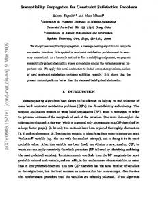
[10] these techniques were formally compared concerning their pruning power. The paper [20] concentrates on theoretical and empirical comparison of singleton consistencies. Figure 9 summarise the results of these and other papers concerning pruning power of basic consistency techniques that are applicable to solving real-life problems.
NIC
SRPC
SAC
PIC
RPC
AC
Strong PC Figure 9: Comparison of pruning power of consistency techniques. A→B means that A is strictly stronger than B (A removes more inconsistencies than B), dashed line means incomparable techniques.
4
Non-binary and global constraints
In Section 2 we mentioned that arbitrary CSP can be translated to an equivalent binary CSP and the filtering techniques surveyed in Section 3 were designed for binary CSP. However, conversion to a binary CSP is sometime/often impracticable and thus consistency notions and techniques are being extended to non-binary constraints [5-8]. Generalised arc consistency. The notion of arc consistency can be simply extended to non-binary constraints, then we are speaking about generalised arc consistency. The constraint is generalised arc consistent (GAC) if for any value of the variable in the constraint there exist values for the other variables in the constraint such that the tuple satisfies the constraint. AC-3 algorithm can be naturally extended to make the constraint network generalised arc consistent and, in fact, this is the most widely used technique in the current constraint satisfaction packages. Instead of revising the binary arc, this algorithm revises the hyper-arcs. For example if the domain of the variable A is changed then the revision of the constraint A+B=C is done by calling the following two functions: C←A+B, B←C-A. Usually, instead of remembering the hyper-arcs in the queue for rerevisions, this algorithm remembers the variables that domain has been changed. Then, the algorithm calls the revision procedures connected to these variables. This approach gives the algorithm enough flexibility necessary for integration of user defined filtering algorithms and, therefore, it is the most common algorithm provided by the constraint satisfaction packages.
GAC-schema. Arc consistency algorithms presented in Section 3 were designed for binary constraints. In [5] a new schema for generalised arc consistency were proposed based on AC-7 algorithm. In [8], an instantiation of this schema was proposed to achieve arc consistency on global constraints. Global constraints. The disadvantage of generalised arc consistency algorithms is decreasing efficiency with growing cardinality of the constraint. As shown in [21], special filtering algorithms can be designed for particular constraints that achieve the same level of consistency but are more time and space efficient thanks to exploiting semantic information about the constraint. Such special constraints are usually called global constraints. They can be often decomposed to simpler (binary) constraints [13,18] but then the same consistency technique, say AC, has lower pruning power and therefore such decomposition often does not pay-off. Several groups of global constraints were proposed motivated by real-life problems [2].
5
Propagation in practice
After surveying the basic filtering techniques used to reduce domains of binary and non-binary constraints, let us now describe some less obvious techniques how the constraint propagation can be improved and how the filtering techniques should be applied to solve real-life problems. The discussed techniques are derived from observations of the author and others so they have more or less experimental nature. Disjunction. Appearance of the disjunctive constraint in the problem formulation usually causes problems because of weak propagation through such constraint. Let us illustrate it with a simple example. Assume that variable x has a domain -10,…,10 and there is a disjunctive constraint (x≤-5 ∨ x≥5). One may assume (wrongly) that after posting this constraint, the domain of the variable x is reduced to (-10,…,-5) ∪ (5,…,10). Unfortunately, in most constraint systems this is not true and the domain of x stay -10,…,10. This is because propagation through particular constraint in the disjunction is activated only when the other constraints are violated. For example, if the domain of x is reduced to say -10,…,3 then x≥5 is not true so the other constraint x≤-5 is activated and the domain of x is reduced further to -10,…, -5. In this clear example, there is a simple solution to increase propagation: instead of the disjunctive constraint one may use the domain constraint x in (inf..-5)\/(5..sup). However, in a more complex disjunction such reformulation may be more complicated or even impossible. Then the solution could be to use a more expensive constructive
disjunction (the domain of the variable is reduced to the union of domains after propagation through the individual constraints in the disjunction) or to design an ad-hoc propagation algorithm. Disjunction in CLP. When constraint logic programming (CLP) is used as an underlying platform for constraint solving then problems with disjunction become even harder. Logic programming provides alternative clauses to model disjunction and many CLP users apply this approach when modelling problems with constraints. For example the disjunctive constraint from the previous paragraph is modelled using the following CLP code: disj(X):-X#==5. This means that a constraint X≤-5 is posted when disj(X) is called and if we find later that this is not good then the alternative constraint X≥5 is used. However, the only way how to install the constraint X≥5 is upon backtracking so everything that has been done since the first call to disj(X) is lost. This unwanted behaviour of CLP when defining disjunctive constraint using alternative clauses was first observed in [28] where a solution using the cardinality operator has been proposed. In [26] the idea of cardinality operator is further extended. Nevertheless, note that cardinality operator still suffers from the problem with non-constructive disjunction described in the previous paragraph. Singleton consistency. As mentioned in Section 3, singleton consistency is a very powerful filtering technique close in pruning power to path consistency but resistant from path consistency problems. Unfortunately like other more powerful consistency techniques, achieving singleton consistency is not cheap in terms of time. Therefore, it is not practical to maintain full singleton consistency during labelling. On the other hand, implementation of singleton arc consistency algorithm is almost for free, it is a combination of labelling, achieving arc consistency, and tabling variables' domains. Note also that opposite to many other consistency techniques, the implementation of SAC does not require changes inside the constraint satisfaction engine but it can be done at a metalevel. We see several ways how singleton consistency can be applied to improve domain filtering. First, it is possible to make the constraint satisfaction problem singleton consistent just once before labelling. This reduces domains more than simple AC while keeping reasonable time complexity. If achieving full SAC is too expensive (and this could be pretty often in large-scale real-life problems) then it is still possible to use SAC in a limited way. In particular, it is possible to apply SAC to selected variables that
somehow determine the solution space. Reducing some domains using SAC can then be propagated to other variables using standard AC. Note that this limited SAC can be applied within labelling as well to achieve a weaker form of maintaining singleton consistency. Maintaining limited singleton consistency can also be used during prototyping a constraint model. It is much easier to implement singleton consistency then to design a special propagation algorithm (global constraint). Thus, singleton consistency (SC) can be used to test if applying stronger consistency over a particular set of variables pays off. If the answer is yes then it is possible to design a special ad-hoc filtering algorithm with similar pruning power as SC but more time efficient than SC. Redundant constraints. Usually, when the user formulates a problem, only the necessary constraints are included in the model. Redundant constraints, i.e., the constraints that can be derived from other constraints are often avoided. This is because redundant constraints do not contribute to the solution set (their presence in the model does not shrink the solution set), and moreover, they increase overhead. On the other side, adding redundant constraints may further reduce domains and, consequently, speed up search. Let us illustrate improved propagation with redundant constraints using a simple CSP. Assume there are four variables x1,x2,x3,x4 with domains 0,…,5, two variables y1,y2 with domains 3,…,8 and constraints x1+x2=y1, x3+x4=y2, x1+x2+x3+x4=z. Visible the domain for z should be 6,…,16 but the propagation infers the domain 0,…, 25. If a redundant constraint y1+y2=z is added then we get the expected domain for z. Dual models. In Section 2 we discussed a dual encoding when converting a non-binary CSP to a binary CSP. In a real-life problem there also typically exist two dual encodings modelling the same problem. In these encodings the constraints are swapped for the variables and vice versa. Let us illustrate dual models using a well-known n-queens problem, where the task is to place n queens onto a n×n chessboard in such a way that the queens are not in conflict. One may choose rows as variables and the constraints describe consistent columns for the queens. Or it is possible to use columns as variables and the constraints describe the compatible rows. Both encodings are fully interchangeable and typically only one of then is chosen to model the problem. However, if both models are used in parallel, we can achieve better pruning. Naturally, there must be special constraints that connect the variables of both models, e.g. in case of n-queens the following constraint can be used: row(i)=j ⇔ column(j)=i. Using both primal and dual model can significantly improve domain reduction, e.g. we get a solution
five times faster for 200 queens when primal and dual encoding was used together. However, one must be very careful about combining both encodings because adding more (redundant) constraints increases overheads of propagation. Sometime this overhead wipes the advantage of better domain filtering and sometimes there is no additional pruning when a dual model is used together with the primal one. Symmetries. Removing inconsistent values from the variables' domains is the main task of constraint propagation. Sometimes, we can improve this propagation by removing symmetrical solutions, i.e., the solutions that can be achieved from another solution by swapping the values of some variables. See Figure 10 for two symmetries in n-queens problem (for simplicity reasons we do not discuss rotation in the n-queens problem).
Figure 10: Horizontal (left) and vertical (right) symmetrical solution to the n-queens problem achieved by mirroring the chessboard over the horizontal and vertical axes.
Symmetry divides the set of possible assignments into equivalence classes. If the search algorithm proves that there is no solution in some class then we do not need to explore the equivalent classes because there is no solution as well. Thus, we can exploit symmetry of the problem to improve domain pruning. Assume that we found that the queen in the first column could not be placed to the first row. Using a horizontal symmetry we can deduce that this queen cannot be placed to the last row as well. This symmetry can be encoded using the following constraint row(1)≤n/2, i.e., the queen in the first column must be placed in the top half of the board. Note that this constraint removes the horizontal symmetry. The vertical symmetry can be removed by using a constraint row(1)