Chapter 1 THEORY AND PRACTICE OF THE MINIMUM SHIFT DESIGN PROBLEM Luca Di Gaspero1 , Johannes G¨artner2 , Guy Kortsarz3 , Nysret Musliu4 , Andrea Schaerf1 and Wolfgang Slany5 1 DIEGM, University of Udine – via delle Scienze 208, I-33100 Udine, Italy
{l.digaspero,schaerf}@uniud.it 2 Ximes Inc – Schwedenplatz 2/26, A - 1010 Wien, Austria
[email protected] 3 Computer Science Department, Rutgers University – Camden, NJ 08102, USA
[email protected] 4 Inst. of Inf. Systems, Vienna University of Technology – A-1040 Wien, Austria
[email protected] 5 Inst. for Software Technology, Graz University of Technology – A-8010 Graz, Austria
[email protected]
Abstract
The min-S HIFT D ESIGN problem is an important scheduling problem that needs to be solved in many industrial contexts. The issue is to find a minimum number of shifts and the number of employees to be assigned to these shifts in order to minimize the deviation from the workforce requirements. Our research considers both theoretical and practical aspects of the minS HIFT D ESIGN problem. First, we establish a complexity result by means of a reduction to a network flow problem. The result shows that even a logarithmic approximation of the problem is NP-hard. However, the problem becomes polynomial if the issue of minimizing the number of shifts is neglected. On the basis of these results, we propose a hybrid heuristic for the problem which relies on a greedy construction phase, based on the network flow analogy, followed by a local search algorithm that makes use of multiple neighborhood relations. An experimental analysis on structured random instances shows that the hybrid heuristic clearly outperforms an existing commercial implementation and highlights the respective merits of the composing heuristics for different performance parameters.
Keywords:
Workforce scheduling, hybrid algorithms, local search, greedy heuristics
2
L. Di Gaspero, J. G¨ artner, G. Kortsarz, N. Musliu, A. Schaerf & W. Slany
Introduction The typical process of planning and scheduling a workforce in an organization is inherently a multi-phase activity [18]. First, the production or the personnel management have to determine the temporal staff requirements, i.e., the number of employees needed for each timeslot of the planning period. Afterwards, it is possible to proceed to determine the shifts and the total number of employees needed to cover each shift. The final phase consists in the assignment of the shifts and days-off to employees. In the literature, there are mainly two approaches to solve the latter two phases. The first approach consists of solving the shift design and the shift assignment phases as a single problem (e.g., [8, 10]). A second approach, instead, proceeds in stages by considering the design and the assignment of shifts as separate problems [1, 13, 14]. However, this approach does not ensure that it will be possible to find a good solution to the assignment problem after the shift design stage. In this work we focus on the problem of designing the shifts. We propose the min-S HIFT D ESIGN formulation where the issue is to find a minimum set of work shifts to use (hence the name) and the number of workers to assign to each shift, in order to meet (or minimize the deviation from) pre-specified staff requirements. The selection of shifts is subject to constraints on the possible start times and the lengths of shifts, and an upper limit for the average number of duties per week per employee. Our work is motivated by practical considerations and differs from other literature dealing with similar problems since we explicitely aim at minimizing the number of shifts. The latter leads to schedules that are easier to read, check, manage and administer. The original formulation of the problem arose in a project at Ximes Inc, a consulting and software development company specializing in shift scheduling. An initial solver for this problem was implemented in a software endproduct called OPA (‘OPerating hours Assistant’) and presented in [15]. The paper is organized as follows. After having formally introduced the problem statement and the relevant related work on the subject (Sect. 1.1), we establish the complexity of the min-S HIFT D ESIGN problem by means of a reduction to a Network Flow problem, namely the cyclic multi-commodity capacitated fixed-charge min-C OST max-F LOW problem [3, Prob. ND32, page 214]. The precise relation between the two problems is shown in Section 1.2. As we will show, even a logarithmic approximation of the problem is NPhard. However, if the issue of minimizing the number of shifts is neglected, the resulting problem becomes solvable in polynomial time. Then, we introduce a hybrid heuristic for solving the problem that is inspired by the relation between the min-S HIFT D ESIGN and the min-C OST max-F LOW problems. The algorithm relies on a greedy solution construction phase, based
Theory and practice of the minimum shift design problem
3
on the min-C OST max-F LOW analogy, followed by a local search algorithm that makes use of the Multi-Neighborhood Search approach [5]. The heuristic solver is presented in Section 1.3. In Section 1.4 we compare the performances of the proposed heuristic solver with OPA. The outcome of the comparison shows that our heuristic significantly outperforms the previous approach. Finally, in Section 1.5 we provide some discussion.
1.
Problem Statement
The minimum shift design problem (MSD) consists in the selection of which work shifts to use and how many people to assign to each such shift in order to meet pre-specified workforce requirements. The requirements are given for d planning days D = {1, . . . , d} (the socalled planning horizon), where a planning day can start at a certain time on a regular calendar day, and ends 24h later, usually on the next calendar day. Each planning day j is split into n equal-size smaller intervals ti = [τi , τi+1 ), called timeslots, which have the same length h = kτi+1 − τi k ∈ R expressed in minutes. The time point τ1 on the first planning day represents the start of the planning horizon, whereas time point τn+1 on the last planning day is the end of the planning horizon. In this work we deal with cyclic schedules, thus τn+1 of the last planning day coincides with τ1 of the first planning day of the next cycle, and the requirements are repeated in each cycle. For each timeslot ti of a day j of a cycle, we are given an optimal number of employees bij , representing the number of persons needed at work in that timeslot. An example of workforce requirements with d = 7 is shown in Table 1.1, where the planning days coincide with calendar days (for the rest of this document we will use the term ‘day’ when referring to planning days unless stated otherwise). In the table, the days are labeled ‘Mon’, ‘Tue’, etc. and, for conciseness, timeslots with the same requirements are grouped together (the example is adapted from a real call-center problem). In this problem we are interested in determining a set of shifts for covering the workforce requirements. Each shift s = [σs , σs + λs ) is characterized by two values σs and λs that determine the starting time and the length of the shift, respectively. Since we are dealing with discrete time slots, for each shift s, the variables σs can assume only the τi values defined above, and the variables λs are constrained to be a multiple of the timeslot length h. The set of all possible shifts is denoted by S. When designing shifts, not all starting times are feasible, neither are all lengths allowed. For this reason, the problem statement also includes a collection of shift types V = {v1 , . . . vr }, each of them characterized by the
4
L. Di Gaspero, J. G¨ artner, G. Kortsarz, N. Musliu, A. Schaerf & W. Slany Start 00:00 06:00 08:00 09:00 10:00 11:00 14:00 16:00 17:00 22:00
Table 1.1.
End Mon Tue Wen Thu Fri Sat Sun 06:00 5 5 5 5 5 5 5 08:00 2 2 2 6 2 0 0 09:00 5 5 5 9 5 3 3 10:00 7 7 7 13 7 5 5 11:00 9 9 9 15 9 7 7 14:00 7 7 7 13 7 5 5 16:00 10 9 7 9 10 5 5 17:00 7 6 4 6 7 2 2 22:00 5 4 2 2 5 0 0 24:00 5 5 5 5 5 5 5
Sample workforce requirements.
Shift type M (morning) D (day) A (afternoon) N (night)
Table 1.2.
min s 05:00 09:00 13:00 21:00
max s 08:00 11:00 15:00 23:00
min l 07:00 07:00 07:00 07:00
max l 09:00 09:00 09:00 09:00
An example of shift types
earliest and the latest starting times (denoted by min s (vk ) and max s (vk ), respectively), and a minimum and maximum length of its shifts (denoted by min l (vk ) and max l (vk )). Each shift s belongs to a unique shift type, therefore its starting time and length are constrained to lie within the intervals defined by its type. We denote the shift type relation with K(s) = vk . A shift s that belongs to the type vk is a feasible shift if min s (vk ) ≤ σs ≤ max s (vk ) and min l (vk ) ≤ λs ≤ max l (vk ). Table 1.2 shows an example of a set of shift types together with the ranges of allowed starting times and lengths. The times are expressed in the format hour:minute. The shift types together with the time granularity h determine the quantity m = |S| of possible shifts. For example, assuming a timeslot length of 15 minutes, there are m = 360 different shifts belonging to the types of Table 1.2. The goal of the min-S HIFT D ESIGN problem is to select a set of q feasible shifts Q = {s1 , s2 , . . . , sq } and to decide how many people xj (s) ∈ N are going to work in each shift s ∈ Q for each day j, so that bij people will be present at each timeslot ti of the day. If we denote the collection of shifts that include the timeslot ti with Sti ⊆ Q, a feasible Psolution consists of d numbers xj (s) assigned to each shift s, so that lij = s∈St xj (s) is equal to bij . In i other words, we require that the number of workers present at time ti , for all values of i and for all days j, meets the staffing requirements. In practical cases, however, this constraint is relaxed, so that small deviations are allowed. To this aim, each solution of the MSD problem is evaluated
5
Theory and practice of the minimum shift design problem Start 06:00 08:00 09:00 14:00 22:00
Table 1.3.
Type M M D A N
Length 08:00 08:00 08:00 08:00 08:00
Mon 2 3 2 5 5
Tue 2 3 2 4 5
Wed 2 3 2 2 5
Thu 6 3 4 2 5
Fri 2 3 2 5 5
Sat 0 3 3 0 5
Sun 0 3 2 0 5
A solution to the min-S HIFT D ESIGN problem
16
required designed
14
12
10
8
6
4
2
0 Mon
Tue
Figure 1.1.
Wed
Thu
Fri
Sat
Sun
Mon
A pictorial representation of the solution in Table 1.3
by means of an objective function to be minimized. The objective function is a weighted sum of three main components. The first and second components are the staffing excess and shortage, namely, the sums F1 (Q, x) = Pd Pn Pd Pn j=1 i=1 max{lij − bij , 0} and F2 (Q, x) = j=1 i=1 max{bij − lij , 0}. The third component of the objective function is the number of shifts selected F3 (Q, x) = |Q|. The MSD problem is genuinely a multi objective optimization problem in which the criteria have different relative importance depending on the situation. Therefore, the weights of the three Fi components depend on the instance at hand and can be adjusted interactively by the user. A solution to the problem in Table 1.1 is given in Table 1.3 and is pictorially represented in Figure 1.1. Notice that this solution is not perfect. For example, there is a shortage of workers every day in the timeslot 10:00–11:00, represented by the thin white peaks in the figure. Conversely, on Saturdays there is an excess of one worker in the period 09:00–17:00. The values of the objectives Fi are the following. The shortage of employees F1 is 15 person-hours, the excess of workers F2 is 7 person-hours, and the number of shifts used, F3 , is 5, as listed in Table 1.3.
6
L. Di Gaspero, J. G¨ artner, G. Kortsarz, N. Musliu, A. Schaerf & W. Slany
Related work Though there is a large literature on shift scheduling problems (see, e.g., [12] for a recent survey), the larger body of work is devoted to the problem of allocation resources to shifts, for which network flow techniques have, among others, been applied (e.g., [1, 2]). Heuristics for a shift selection problem that has some similarity with minS HIFT D ESIGN have been studied by Thompson [17]. In [2], Bartholdi et al. noticed that a problem similar to min-S HIFT D ESIGN can be translated into a min-C OST max-F LOW problem (which is a polynomial problem, see, e.g., [16]) and thus efficiently solved. The translation can be applied under the hypothesis that the requirement of minimizing the number of selected shifts is neglected and the costs for assignments that do not fulfill the requirements are linear. To the authors knowledge, the only paper that deals explicitly with the formulation of the min-S HIFT D ESIGN problem considered in this work is a previous paper of Musliu et al. [15], which presents the OPA software. In Section 1.4, we will compare our heuristic solver with the implementation described in [15] by applying it to the set of benchmark instances used in that paper.
2.
Theoretical results
In this section we prove that a restricted version of min-S HIFT D ESIGN is equivalent to the infinite capacities flow problem on a Direct Acyclic Graph with unitary edge costs (UDIF), which, in turn, is a variant of min-C OST maxF LOW problem [3, Prob. ND32, page 214]. First we present the UDIF problem, which is a network flow problem with the following features: (1) Every edge not incident to the sink or to the source, called proper edge, has infinite capacity. Non-proper edges, namely edges incident to the source or to the sink, have arbitrary capacities. (2) The costs of proper edges is 1, whereas the cost of non-proper edges is 0. (3) The underlying flow network is a Direct Acyclic Graph. (4) The goal is, as in the general problem, to find a maximum flow f (e) over the edges (obeying the capacity and flow conservation laws) and, among all maximum flows, to choose the one minimizing the cost of edges carrying non-zero flow. Hence, in this case, the problem is to minimize the number of proper edges carrying nonzero flow (namely, minimizing |{e : f (e) > 0, e is proper}|). Thanks to the equivalency between min-S HIFT D ESIGN and UDIF, a hardness of approximation result for UDIF carries over to min-S HIFT D ESIGN and,
Theory and practice of the minimum shift design problem
7
as we are going to see, we could prove a logarithmic lower bound on these problems. To simplify the theoretical analysis of min-S HIFT D ESIGN, in this section we restrict ourselves to min-S HIFT D ESIGN instances where d = 1 (i.e., workforce requirements are given for a single day only), and no shifts in the collection of possible shifts span over two days, that is, each shift starts and ends on the same day. We also assume that for the evaluation function, the weights for excess and shortage are equal and are much larger than weights for the number of shifts. This effectively gives priority to the minimization of deviation, thereby only minimizing the number of shifts for all those feasible solutions already having minimum deviation. It is useful to describe the shifts via 0 − 1 matrices with the consecutive ones property. A matrix obeys the consecutive ones (c1) property if all entries in the matrix are either 0 or 1 and all the 1 in each column appear consecutively. A matrix A for which the c1 property holds is called a c1 matrix. We now provide a formal description of min-S HIFT D ESIGN by means of c1 matrices as follows. We are given an n × m matrix A in which each column corresponds to a possible shift. Each entry ais in the matrix is either 1 if i is a valid timeslot for shift s or 0 otherwise. Since the set of valid timeslots for a given shift type (and thus for a given shift belonging to a shift type) is made up of consecutive timeslots, A is clearly a c1 matrix. Furthermore, we are given a vector b of length n of positive integers; each entry bi corresponds to the workforce requirement for the timeslot i. Within these settings, the minS HIFT D ESIGN problem can be stated as a system of inequalities: Ax ≥ b with x ∈ Zn , x ≥ 0, where the vectors x correspond to the shift assignments. The optimization criteria are represented as follows. Let Ai be the ith row in A, and kxk1 denote the L1 norm of x. We are looking for a vector x ≥ 0 with the following properties: (1) The vector x minimizes kAx − bk1 (i.e., the deviation from the staffing requirements). (2) Among all vectors minimizing kAx − bk1 , x has a minimum number of non-zero entries (corresponding to the number of selected shifts). Given this formulation of the restricted variant of min-S HIFT D ESIGN it is possible to prove the following result (the detailed proof is contained in [4]).
Proposition 1.1 The restricted one-day noncyclic variant of min-S HIFT D ESIGN where a zero deviation solution exists (i.e., h = 1, all shifts start and finish on the same day, and Ax∗ = b admits a solution), is equivalent to the UDIF problem. The proof proceeds as follows: first a flow matrix F that preserves the solutions of the problem Ax = b is constructed, by means of a regular transforma-
8
L. Di Gaspero, J. G¨ artner, G. Kortsarz, N. Musliu, A. Schaerf & W. Slany
tion of A. Then, after a little post-processing of F, the resulting flow problem becomes an instance of UDIF. It is possible to show that this result can be exploited also for handling workforce shortage and excess (components F1 and F2 of the objective function), by introducing a set of n slack variables yi and solving the problem (A; −I)(x; y) = b. Moreover, if we neglect the problem of minimizing the number of shifts, the problem (A; −I)(x; y) = b can be transformed into a min-C OST max-F LOW (MCMF) problem. This allows us to efficiently find the minimum (weighted) deviation from the workforce requirements, and this idea will be employed in the first stage of our heuristic presented in Section 1.3. We next state that, unless P = NP , there is some constant c < 1 such that approximating UDIF within c ln n−ratio is NP-hard. Since the case of zero excess min-S HIFT D ESIGN is equivalent to UDIF, similar hardness results follow for min-S HIFT D ESIGN as well.
Theorem 1.2 There is a constant c < 1 so that approximating the UDIF problem within c ln n is NP-hard. The proof employs a reduction from the S ET-C OVER problem and is omitted for brevity.
3.
Heuristic solver
Our solution heuristic is divided into two stages, namely a greedy construction for the initial solution and a tabu search procedure [7] that iteratively improves it, which are described in the following subsections. In our experiments we evaluate the behavior of each stage and of the resulting hybrid algorithm, in order to analyze the sensitivity of the tabu search procedure to the starting point used.
Greedy constructive heuristic Based on the equivalence of the (non-cyclic) min-S HIFT D ESIGN problem to UDIF, and the relationship with the min-C OST max-F LOW problem, we propose a new greedy heuristic GreedyMCMF() that uses a polynomial minC OST max-F LOW subroutine (MCMF()). The pseudocode of the algorithm is reported in Figure 1.2. The algorithm is based on the observation that the min-C OST max-F LOW subroutine can easily compute the optimal staffing with minimum (weighted) deviation when slack edges have associated costs corresponding, respectively, to the weights of shortage and excess. Note that, however, the algorithm is not able to simultaneously minimize the number of shifts that are used. Since the MCMF() subroutine cannot consider cyclicity, we must first perform a preprocessing step that determines a good split-off time where the cycle
Theory and practice of the minimum shift design problem
9
function GreedyMCMF(S,b): MSD Solution /* 1. Preprocessing step: where to break cyclicity? */ t := FindBestSplitOffTime(S,b); // Search for a split-off on the 1st day of the cycle /* 2. Greedy part with MCMF subroutine */ f ∗ := MCMF(MSD2Flow(S,b,t)); // Compute best flow so far for MSD instance σ := ShiftsAndWorkforceIn(f ∗ ); // Shifts are edges with flow 6= 0; workforce is edge flow // Cost of the best MSD solution found so far min cost := MSD Eval(σ); Q := ShiftsInUseIn(σ); // Shifts in the current solution T := ∅; // Shifts already tried repeat s := UniformlyChooseAShiftFrom(Q \ T ); // Consider a shift s that is used but not tried yet f := MCMF(MSD2Flow(Q \ {s},b,t)); // Try to solve the problem without shift s σ := ShiftsAndWorkforceIn(f ); // Extract shifts and workforce from flow solution // Compute the cost of the current solution current cost := MSD Eval(σ); if current cost < min cost then min cost := current cost; // Solution with one shift less and lower cost f ∗ := f ; // Update the best solution found so far Q := ShiftsInUseIn(σ); // Could be less than Q \ {s} endif T := T ∪ {s}; // Add s to shifts already tried until Q \ T = ∅; // Cycle until no shift to try is left /* 3. Postprocessing step to recover cyclicity, perform a local search with the ExchangeStaff move */ σ := SteepestDescent(ShiftsAndWorkforceIn(f ∗ ), ExchangeStaff); return σ;
Figure 1.2. The Greedy min-C OST max-F LOW (MCMF) subroutine computes a solution for the min-S HIFT D ESIGN (MSD) problem
of d days should be broken. This is done heuristically by calling MCMF() with different starting times chosen between 5:00 and 8:00 on the first day of the cycle (in practice, we can observe that there is usually a complete exchange of workforce between 5:00 and 8:00 on the mornings of the first day). All possibilities in this interval are tried while eliminating all shifts that span the chosen starting point when translating from MSD to the network flow instances. The number of possibilities depends on the length of the timeslots of the instance (i.e., the time granularity). The starting point with the smallest cost as determined by MCMF() is used as the split-off time for the rest of the calls to MCMF() in GreedyMCMF. This method has been shown to provide adequate results in practice. In the main loop, the greedy heuristic then removes all shifts that did not contribute to the MSD instance corresponding to the current flow computed with MCMF(). It randomly chooses one shift (without repetitions) and tests whether removal of this shift still allows the MCMF() to find a solution with the same deviation. If this is the case, that shift is removed and not considered anymore, otherwise it is left in the set of shifts used to build the network flow instances, but it will not be considered for removal again. Finally, when no shifts can be removed anymore without increasing the deviation, a final postprocessing step is made to restore cyclicity. It consists of
10 L. Di Gaspero, J. G¨artner, G. Kortsarz, N. Musliu, A. Schaerf & W. Slany a simple repair step performed by a fast steepest descent runner that uses the ExchangeStaff neighborhood relation (see below). The runner selects at each iteration the best neighbor, with a random tie-break in case of same cost. It stops as soon as it reaches a local minimum, i.e., when it does not find any improving move. c 1995 – 2001 IG As our MCMF() subroutine, we use CS2 version 3.9 ( Systems, Inc., http://www.avglab.com/andrew/soft.html), an efficient implementation of a scaling push-relabel algorithm [9], slightly edited to be callable as a library.
Multi-Neighborhood Search for Shift Design The second stage of the proposed heuristic is a local search procedure based on multiple neighborhood relations. We first define the search space, then describe the set of neighborhood relations for the exploration of this search space, followed by the search strategies we employ.
Search space. We consider as a state for MSD a pair (Q, X) made up of a set of shifts Q = {s1 , s2 , . . .} and their staff assignment X = {x1 , x2 , . . .}. The shifts of a state are split into two categories: Active shifts: at least one employee is assigned to a shift of this type on at least one day. Inactive shifts: no employees are assigned to a shift of this type on any day. These shifts does not contribute to the solution and to the objective function. Their role is explained later. More Pd formally, we say that a shift si ∈ Q is active (resp. inactive) if and only if j=1 xj (si ) 6= 0 (= 0).
Neighborhood exploration. In this work we consider three different neighborhood relations that are combined in the spirit of the Multi-Neighborhood search described in [5]. In short, the Multi-Neighborhood Search consists in a set of operators for automatically combining basic neighborhoods and in a set of strategies for combining algorithms (called runners) based on different neighborhoods. The motivation for applying a combination of neighborhoods comes from the observation that for most problems there is more than one natural neighborhood that deserves to be investigated. Furthermore, using different neighborhoods or algorithms in different phases of the search increases diversification, thereby improving the performance of the local search metaheuristics. The way the neighborhoods are employed during the search is explained later. In the following we formally describe each neighborhood relation by means of the attributes needed to identify a move, the preconditions for its
Theory and practice of the minimum shift design problem
11
applicability, the effects of the move and, possibly, some rules for handling special cases. Given a state (Q, X) of the search space the types of moves considered in this study are the following: ChangeStaff (CS): The staff of a shift si is increased or decreased by one employee, that is either x0j (si ) := xj (si ) + 1, or x0j (si ) := xj (si ) − 1. If si is an inactive shift and the move increases its staff, then si becomes active and a new randomly created inactive shift of type K(si ) is inserted (distinct from the other shifts). ExchangeStaff (ES): One employee in a given day is moved from one shift si1 to another one of the same type (say si2 ), i.e., x0j (si1 ) := xj (si1 ) − 1 and x0j (si2 ) := xj (si2 ) + 1. If si2 is an inactive shift, si2 becomes active and a new random distinct inactive shift of type K(si1 ) is inserted (if such a distinct shift exists). If the move makes si1 inactive then, in the new state, the shift si1 is removed from the set Q. ResizeShift (RS): The length of a shift si is increased or decreased by one time slot, either on the left-hand side or on the right-hand side of the interval. For this kind of move we require that the shift s0i , obtained from si by the application of the move must be feasible with respect to the shift type K(si ). We denote with δ the size modification to be applied to the shift si , that is δ = +1 when the shift is enlarged by one timeslot and δ = −1 when the shift is shrunk. If the action should be performed on the left-hand side of si we have that σi0 := σi − δh and λ0i := λi + δh. Conversely, if the move should take place on the right-hand side σi remains unchanged and λ0i := λi + δh. In a previous work, Musliu et al. [15] define many neighborhood relations for this problem including CS, ES, and a variant of RS. In this work, instead, we restrict ourselves to the above three relations for the following two reasons: First, CS and RS represent the most atomic changes, so that all other move types can be built as chains of moves of these two. For example, an ES move can be obtained by a pair of CS moves that delete one employee from the first shift and add one to the other shift. Secondly, even though ES can be seen as a composition of two more basic moves as just explained, we employ it because it turned out to be very effective for the search, especially in combination with the concept of inactive shifts. In fact, the transfer of one employee from a shift to a similar one makes a very
12 L. Di Gaspero, J. G¨artner, G. Kortsarz, N. Musliu, A. Schaerf & W. Slany small change to the current state, thus allowing for fine grained adjustments that could not effectively be achieved by the other move types. Inactive shifts allow us to insert new shifts and to move staff between shifts in a uniform way. This approach limits the creation of new shifts only to the current inactive ones, rather than considering all possible shifts belonging to the shift types (which are many more). The possibility of creating any legal shift is rescued if we insert as many (distinct) inactive shifts as compatible with the shift type. Experimental results, though, show that there is a trade-off between computational cost and search quality which seems to have its best compromise in having two inactive shifts per type.
Search strategies. For the purpose of analyzing the behavior of the local search heuristic alone, we provide also a mean to generate a random initial solution for the local search algorithm. That is, we create a fixed number of random distinct active and inactive shifts for each shift type. Afterwards, for the active shifts, we assign a random number of employees for each day. In detail, the parameters needed to build a solution are the number of active and inactive shifts for each shift type and the range of the number of employees per day to be assigned to each random active shift. For example, in the experimental session described in Section 1.4, we build a solution with four active and two inactive shifts per type, with one to three employees per day assigned to each active shift. If the possible shifts for a given shift type are less than six, we reduce the generated shifts accordingly, giving precedence to the inactive ones. The proposed local search heuristic is based on tabu search, which turned out to give the best results in a preliminary experimental phase. However, we have developed and experimented also with a set of solvers based on the hill climbing and simulated annealing meta-heuristics. A full description of tabu search is out of the scope of this paper and we refer to [7] for a general introduction. We describe later in this section its specialization to the MSD problem. We employ the three neighborhoods defined above selectively in various phases of the search, rather than exploring all neighborhoods at each iteration. In detail, we combine the neighborhood relations CS, ES, and RS, according to the following scheme made of compositions and interleaving (through the, so-called, token-ring search strategy). That is, our algorithm interleaves three different tabu search runners using the ES move alone, the RS move alone, and the set-union of the two neighborhoods CS and RS, respectively. The token-ring search strategy implemented is the same as that described in [5], i.e., the runners are invoked sequentially and each one starts from the best state obtained from the previous one. The overall process stops when a full round of all of them does not find an improvement. Each single runner
Theory and practice of the minimum shift design problem
13
stops when it does not improve the current best solution for a given number of iterations. The reason for using only some of the possible neighborhood relations introduced in [15] is not related to the saving of computational time, which could be obtained in other ways, for example by a clever ordering of promising moves, as done in the cited paper. The main reason, instead, is the introduction of a suitable degree of diversification in the search. In fact, certain move types would be selected very rarely in a full-neighborhood exploration strategy, even though they could help to escape from local minima. For example, we experimentally observe that a runner that uses all the three neighborhood relations combined by means of the union operator would almost never perform a CS move that deteriorates the objective function. The reason for this behavior is that such a runner can always find an ES move that deteriorates the objectives by a smaller amount, even though the CS move could lead to a more promising region of the search space. This intuition is confirmed by the experimental analysis that shows that our results are much better than those in [15]. This composite solver is further improved by making two adjustments to the final state of each runner, the results of which is then handed over as the initial state to the following runner, as follows: Identical shifts are merged into one. When RS moves are used, it is possible that two shifts become identical. This is not checked by the runner after each move as it is a costly operation, and is therefore left to this inter-runner step. Inactive shifts are recreated: the current inactive shifts are deleted, and new distinct ones are created at random in the same quantity. This step, again, is meant to improve the diversification of the search algorithm. Concerning the prohibition mechanism of tabu search, for all three runners, the size of the tabu list is kept dynamic by assigning to each move a number of tabu iterations randomly selected within a given range. The ranges vary for the three runners, and were selected experimentally. The ranges are roughly suggested by the cardinality of the different neighborhoods, in the sense that a larger neighborhood deserves a longer tabu tenure. According to the standard aspiration criterion defined in [7], the tabu status of a move is dropped if it leads to a state better than the current best. As already mentioned, each runner stops when it has performed a fixed number of iterations without any improvement (called idle iterations). For practical reasons, in order to avoid the setting of parameters by an enduser, tabu lengths and idle iterations are selected once for all, and the same values were used for all the instances. The selection turned out to be robust
14 L. Di Gaspero, J. G¨artner, G. Kortsarz, N. Musliu, A. Schaerf & W. Slany
Table 1.4.
Parameter Tabu range
TS(ES) 10-20
TS(RS) 5-10
Idle iterations
300
300
TS(CS∪RS) 20-40 (CS) 5-10 (RS) 2000
Tabu search parameter settings
enough for all tested instances. The choice of parameter values is reported in Table 1.4.
4.
Computational results
In this section, we describe the results obtained by our solver on a set of benchmark instances. First, we introduce the instances used in this experimental analysis, then we illustrate the performance parameters that we want to highlight, and finally we present the outcomes of the experiments.
Description of the Sets of Instances The instances consist of three different sets, each containing thirty randomly generated instances. Instances were generated in a structured way to ensure that they look as similar as possible to real instances while allowing the construction of arbitrarily difficult instances. Set 1 contains the 30 instances that were investigated and described in [15]. They vary in their complexity and we mainly include them to be able to compare the solvers with the results reported in that paper for the OPA implementation. Basically, these instances were generated by constructing feasible solutions with some random elements as they usually appear in real instances, and then taking the resulting staffing numbers as workforce requirements. This implies that a very good solution with zero deviation from workforce requirements is known. Note that our solver could find even better solutions for several of the instances, so these reference solutions may be suboptimal. Nevertheless, we refer in the following to the best solutions we could come up with for these instances as the “best known” solutions. Set 2 contains instances that are similar to those of Set 1. However, in this case the reference solutions of instances 1 to 10 were constructed to feature 12 shifts, those of instances 11 to 20 to feature 16 shifts, and those of instances 21 to 30 to feature 20 shifts. This allows us to study the relation between the number of shifts in the “best known” solutions and the running times of the solver using the different settings. While knowing these “best known” solutions eases the evaluation of the proposed solver in the different settings, it also might form a biased preselection toward instances where zero deviation solutions exist for sure, thereby letting the solver behave in ways that are unusual for instances for which no such so-
Theory and practice of the minimum shift design problem
15
lution can be constructed. For this reason, the remaining set is composed of instances where with high likelihood solutions without deviations do not exist: Set 3 contains instances without reference solutions. They were constructed with the same random instances generator as the previous sets but allowing the constructed solutions to contain invalid shifts that deviate from normal starting times and lengths by up to 4 timeslots. The number of shifts is similar to those in Set 2, i.e., instances 1 to 10 feature 12 shifts (invalid and valid ones), and so on. This construction ensures that it is unlikely that there exist zero deviation solutions for these instances. It might also be of interest to see whether a significant difference in performance for the solver employing the different settings can be recognized compared to Set 2, which would provide evidence that the way Sets 1 and 2 were constructed constituted a bias for the solver. All sets of instances are available in self-describing text files from http: //www.dbai.tuwien.ac.at/proj/Rota/benchmarks.html. A detailed description of the random instance generator used to construct them can be found in [15].
Experimental setting In this work we made two types of experiments, aiming at evaluating two different performance parameters: 1) the average time necessary to reach the best known solution; 2) the average cost value obtained within a time bound. Our experiments have been run on different machines. The local search solvers are implemented in C++ using the E ASY L OCAL ++ framework [6] and they were compiled using the GNU g++ compiler version 3.2.2 on a 1.5 GHz AMD Athlon PC running Linux Kernel 2.4.21. The greedy min-C OST maxF LOW algorithm, instead, was coded in MS Visual Basic and run on a MS Windows NT 4.0 computer. The running times have been normalized according to the DIMACS netflow benchmark (ftp://dimacs.rutgers.edu/pub/netflow/benchmarks/c/) to the times of the Linux PC (calibration timings on that machine for above benchmark: t1.wm: user 0.030 sec t2.wm: user 0.360 sec). Because of the normalization the reported running times should be taken as indicatory only. We experiment with the following three heuristic solvers: GrMCMF The GreedyMCMF() algorithm is called repeatedly until the stopping criterion is reached. Since the selection of the next shift to be removed in the main loop of GreedyMCMF() is done randomly, we call the basic heuristic repeatedly and use bootstrapping as described in [11] to compute expected values for the computational results (counting the
16 L. Di Gaspero, J. G¨artner, G. Kortsarz, N. Musliu, A. Schaerf & W. Slany preprocessing step only once for each instance since it computes the same split-off time for all runs). TS The tabu search procedure is repeated several times starting from different random initial solutions. The procedure is stopped either when the time granted has elapsed or when the best solution is reached. Each round of the tabu search procedure is allowed to run at most for 10 seconds. GrMCMF+TS The two solvers are combined in a hybrid heuristic by using the solutions delivered by the GreedyMCMF() procedure as initial states for TS trials. In order to maintain diversification, we exploit the non-determinism of GreedyMCMF() to generate many different solutions, and the initial state of each trial of TS is randomly selected among those states.
Time-to-best results The first experiment evaluates of the running times needed to reach the “best known” solution. We ran the solvers on data Set 1 for 10 trials until they could reach the “best known” solution, and we recorded the running times for each trial. Table 1.5 shows the average times and their standard deviations (between parentheses) expressed in seconds, needed by our solvers to reach the best known solution. The first two columns show the instance number and the best known cost for that instance. The third column reports the cost of the best solution found by the commercial tool OPA. Bold numbers in the second column indicate that the best known solution for this instance was not found by OPA. Dash symbols denote that the best known solution could not be found in any of the 10 trials for those instances. First, note that all three solvers in general produce better results than the commercial tool. In fact, TS always finds the best solution, GrMCMF in 20 cases and GrMCMF+TS in 29 cases out of 30 instances. OPA, instead, could find the best solution only for 17 instances. However, looking at the time performance on the whole set of instances, it is clear that TS is roughly 30 times slower than GrMCMF and 1.5 times slower than the hybrid heuristic. GrMCMF+TS is significantly outperformed by TS only for some few instances for which GrMCMF could not find the best known solution, thus biasing the local search part of the heuristic away from search space near the best known solution. As a general remark, the TS algorithm proceeds by relatively sudden improvements, especially in the early phases of the search, while the behavior of the GrMCMF+TS is much smoother (we omit graphs showing this for brevity). Thus, it is easier to predict the benefits of letting GrMCMF+TS run for a longer period of time compared to TS alone.
17
Theory and practice of the minimum shift design problem Instance
Best
1 2 3 4 5 6 7 8 9 10 11 12 13 14 15 16 17 18 19 20 21 22 23 24 25 26 27 28 29 30
480 300 600 450 480 420 270 150 150 330 30 90 105 195 180 225 540 720 180 540 120 75 150 480 480 600 480 270 360 75
OPA [15] 480 390 600 1,170 480 420 570 180 225 450 30 90 105 390 180 375 1,110 720 195 540 120 75 540 480 690 600 480 270 390 75
GrMCMF 0.07 — 0.11 — 0.20 0.06 1.13 — 3.53 — 0.21 0.25 0.35 — 0.04 — — 1.71 — 0.11 0.28 0.65 6.19 0.11 — 1.50 0.07 2.24 — 0.26
(0.00) (—) (0.01) (—) (0.16) (0.01) (1.10) (—) (2.63) (—) (0.00) (0.00) (0.13) (—) (0.00) (—) (—) (1.30) (—) (0.01) (0.00) (0.45) (2.91) (0.04) (—) (1.14) (0.00) (0.94) (—) (0.00)
TS 5.87 16.41 8.96 305.37 5.03 2.62 10.25 18.98 11.85 66.05 1.79 6.10 7.20 561.99 0.89 198.50 380.72 7.72 38.33 15.24 6.19 3.67 19.16 2.85 503.40 9.59 4.02 9.25 20.59 2.78
(4.93) (9.03) (5.44) (397.71) (2.44) (0.99) (5.77) (15.70) (2.28) (41.27) (0.37) (1.50) (2.30) (404.33) (0.11) (117.84) (467.64) (2.89) (20.72) (6.18) (1.32) (0.80) (10.92) (0.38) (136.17) (6.80) (0.71) (7.67) (17.20) (0.30)
GrMCMF+TS 1.06 40.22 1.64 108.29 1.75 0.62 6.95 10.64 8.85 84.11 0.85 3.84 3.82 60.97 0.40 151.78 288.42 7.32 31.12 1.69 2.18 3.80 22.15 1.44 — 9.20 2.34 3.81 10.00 1.95
(0.03) (27.93) (0.05) (75.32) (1.43) (0.02) (2.88) (0.56) (1.56) (99.85) (0.02) (0.10) (0.09) (51.08) (0.01) (125.88) (27.58) (3.79) (17.99) (0.07) (0.11) (0.86) (15.34) (0.72) (—) (6.20) (0.06) (0.62) (4.92) (0.01)
Table 1.5. Times to reach the best known solution for Set 1. Data are averages and standard deviations (between parentheses) for 10 trials.
Starting local search from the solution provided by GrMCMF has also an additional benefit in terms of the increase of robustness, roughly measured by the standard deviations of the running times. In fact, for this set of instances, while the standard deviation for TS is about 50% of the average running time, this value decreases to 35% for GrMCMF+TS. The behavior of the GrMCMF solver is similar to the one of the hybrid heuristic and the standard deviation is about 35% of the average running time.
Time-limited experiments Moving to the time-limited experiments, we perform two experiments on the different sets of instances. The first experiment with limited running times aims at showing how the solver scales up with respect to the optimum number of shifts. For this purpose we recorded the cost values of 100 runs of our solvers with the different settings on the instances of Sets 1 and 2, for which
GreedyMCMF TS GrMCMF+TS
0
0.02
0.04
0.06
0.08
0.1
0.12
0.14
18 L. Di Gaspero, J. G¨artner, G. Kortsarz, N. Musliu, A. Schaerf & W. Slany
8
Figure 1.3.
10
12
14
16
18
20
Aggregated normalized costs for 10s time-limit on data Sets 1 and 2.
the value of a good solution is known. The runs were performed by granting to each trial a time-limit of 10 seconds. The results of the experiment are grouped on the basis of the instance size and are shown in Figure 1.3. The X axis of the figure shows the number of shifts in the best known solution where results on instances with the same number of shifts are clustered together. The Y axis shows normalized costs, obtained by dividing the difference between the average cost and the best cost by the latter value. In other words, each cost y obtained on instance i, for which the best known cost is besti , is transformed by means of the function i fi (y) := y−best besti . The graph presents the data as box-and-whiskers plots, i.e., it shows the range of variation (the interval [fi (min-costi ), fi (max-costi )]), denoted by the dashed vertical line, and the frequency distribution of the solutions. The latter measure is expressed by means of a boxed area featuring the range between the 1st and the 3rd quartile of the distribution (accounting for 50% of the frequency). The horizontal line within the box denotes the median of the distribution and the notches around the median indicate the range for which the difference of medians is significant at a probability level of p < 0.05. The figure shows that, for short runs, the hybrid solver is superior to GrMCMF and TS alone, both in terms of solution quality and robustness: the ranges of variation are shorter and the frequency boxes are tinier. Looking at these results from another point of view, it is worth noting that GrMCMF+TS is able to find more low-cost (and even min-cost) solutions that are significantly better than those found by TS and GrMCMF. Furthermore, it is apparent that the hybrid heuristic scales better than its components, since the
Theory and practice of the minimum shift design problem Instance 1 2 3 4 5 6 7 8 9 10 11 12 13 14 15 16 17 18 19 20 21 22 23 24 25 26 27 28 29 30
GrMCMF 2,445.00 (0.00) 7,672.59 (34.92) 9,582.14 (32.97) 6,634.40 (39.67)† 10,053.75 (41.58) 2,082.17 (17.31)† 6,075.00 (0.00) 9,023.46 (45.78) 6,039.18 (23.36)† 2,968.95 (16.88) 5,511.43 (26.11) 4,231.96 (51.83) 4,669.50 (56.42)† 9,616.55 36.24 11,448.90 (92.21)† 10,785.00 (75.98) 4,746.56 (37.72) 6,769.41 (84.94) 5,183.16 (57.26) 9,153.90 (80.98) 6,072.86 (44.37) 12,932.31 (82.87) 8,384.24 (122.90) 10,545.00 (26.11) 13,204.80 (18.45) 13,152.73 (97.27)† 10,084.94 (24.86)† 10,641.21 (100.81) 6,799.41 71.78 13,770.68 92.32
TS 9,916.35 (3,216.35) 9,582.00 (1,564.39) 12,367.50 (1,576.56) 8,956.50 (2,091.76) 10,311.60 (198.54) 4,712.25 (1,614.34) 12,251.70 (1,553.22) 10,512.60 (1,658.02) 11,640.60 (2,264.50) (4,067.10) 1,226.20 7,888.20 (2,116.61) 11,410.05 (1,510.78) 10,427.55 (1,593.59) 10,130.40 (290.29) 13,563.60 (1,415.06) 11,180.40 (298.02) 11,735.40 (2,253.94) 9,516.60 (1,929.90) 10,825.20 (2,254.98) 12,481.80 (1,834.54) 14,102.55 (1,194.54) 16,418.70 (1,729.19) 9,788.40 (886.01) 11,413.20 (769.58) 14,038.80 (701.17) 17,326.50 (2,421.45) 10,866.60 (651.65) 11,543.40 (675.60) 12,075.30 2,710.45 14,808.60 692.80
19
GrMCMF+TS 2,386.80 (9.60) 7,691.40 (50.95) 9,597.00 (27.14) 6,681.60 (119.70)† 9,996.00 (127.35) 2,076.75 (7.50)† 6,087.00 (16.92) 8,860.50 (55.98) 6,036.90 (28.80)† 3,002.40 (41.49) 5,490.90 (69.86) 4,171.20 (22.23) 4,662.00 (39.77)† 9,660.60 (50.81) 11,445.00 (110.66)† 10,734.00 (62.38) 4,729.05 (38.13) 6,692.40 (54.55) 5,157.45 (51.22) 9,174.90 (62.97) 6,053.55 (32.28) 12,870.30 (63.89) 8,390.40 (72.22) 10,417.80 (79.84) 13,252.20 (100.42) 13,117.80 (114.15)† 10,081.20 (45.91)† 10,603.80 (86.49) 6,690.00 (62.81) 13,723.80 (72.79)
Table 1.6. Results for Set 3: cost values within 1s time-limit. Data are averages and standard deviations (between parentheses) of 100 trials. The best algorithm on each instance is highlighted in boldface; the symbol † denotes the cases for which the difference between the distribution of solutions was not statistically significant (Mann-Whitney test with p < 0.01).
deterioration in the solution quality with respect to the number of shifts grows very slowly and always remains under an acceptable level (7% on the worst case, and about 2% for 75% of the runs). The second time-limited experiment aims at investigating the behavior of the solver when provided with a very short running time on “unknown” instances (we use here the term “unknown” by contrast with the sets of instances constructed around a reference solution). We performed this experiment on the third data set and we recorded the cost values found by our solver over 100 trials. Each trial was granted 1 second of running time, in order to simulate a practical situation in which the user needs a fast feedback from the solver. For this problem, speed is of crucial importance to allow for immediate discussion in working groups and refinement of requirements, especially if such a solver is used during a meeting with customers. Hence, without quick answers, understanding requirements and consensus building is much more difficult.
20 L. Di Gaspero, J. G¨artner, G. Kortsarz, N. Musliu, A. Schaerf & W. Slany In Table 1.6 we report the average and the standard deviation (between parentheses) of the cost values found by each heuristic. In this case the hybrid heuristic performs better than TS on all instances, and it shows a better behavior in terms of algorithm robustness (in fact, the standard deviation of GrMCMF+TS is usually more than an order of magnitude smaller than the one of TS). Moreover, even the GrMCMF achieves better results than the TS heuristic, due to the running time performance of the local search procedure. However, differently from the results of the previous experiment, the hybrid heuristic does not dominate the GrMCMF on all instances. In fact, it is possible to see that GrMCMF+TS finds better results on 15 instances, whereas GrMCMF prevails in 8 cases. On 7 instances there is no clear winner among the two heuristics, and these cases are indicated by the symbol † in the table. The reason of this behavior is related to the amount of running time needed by the local search procedure. Indeed, in another experiment (omitted for brevity) with a higher time-limit, the behavior of the three heuristic tends to be similar to the one observed in the previous experiment, indicating the absence of bias in the construction of sets 1 and 2 of instances.
5.
Conclusions
The min-S HIFT D ESIGN problem is an important shift scheduling problem that arises in many industrial contexts. We provided complexity results for it and designed a hybrid heuristic algorithm composed of a constructive heuristic (suggested by the complexity analysis) and a multi-neighborhood tabu search procedure. This problem appears to be quite difficult in practice, even for small instances, which is also supported by the theoretical results. An important source of hardness is related to the variability in the size of the solution, since dropping this requirement makes the problem solvable in polynomial time. In the experimental part, the hybrid heuristic and its underlying components have been evaluated both in terms of ability to reach good solutions and in quality of solutions reached in fast runs. The outcomes of the comparison show that the hybrid heuristic combines the good features of its components. Indeed, it obtained the best performances in term of solution quality (thanks to the increased thoroughness allowed by tabu search) but with a lower impact on the overall running time. Furthermore, we compare our heuristics with the results obtained with a commercial software as reported [15]. Our hybrid heuristic clearly outperforms this commerical implementation, and thus can be considered as the best general-purpose solver among the other heuristics that were compared to it.
Bibliography
[1] N. Balakrishnan and R.T. Wong. A network model for the rotating workforce scheduling problem. Networks, 20:25–42, 1990. [2] J. Bartholdi, J. Orlin, and H.Ratliff. Cyclic scheduling via integer programs with circular ones. Operations Research, 28:110–118, 1980. [3] M. R. Garey and D. S. Johnson. Computers and Intractability—A guide to NP-completeness. W.H. Freeman and Company, San Francisco, 1979. [4] L. Di Gaspero, J. G¨artner, G. Kortsarz, N. Musliu, A. Schaerf, and W. Slany. The minimum shift design problem: theory and practice. In Giuseppe Di Battista and Uri Zwick, editors, Proc. of the 11th Annual European Symposium on Algorithms (ESA 2003), number 2832 in Lecture Notes in Computer Science, pages 593–604. Springer-Verlag, BerlinHeidelberg, 2003. ISBN 3-540-20064-9. [5] L. Di Gaspero and A. Schaerf. Multi-neighbourhood local search with application to course timetabling. In E. Burke and P. De Causmaecker, editors, Lecture Notes in Computer Science, number 2740 in Lecture Notes in Computer Science, pages 263–278. Springer-Verlag, BerlinHeidelberg, 2003. ISBN 3-540-40699-9. [6] L. Di Gaspero and A. Schaerf. E ASY L OCAL ++: An object-oriented framework for flexible design of local search algorithms. Software Practice & Experience, 33(8):733–765, July 2003. [7] F. Glover and M. Laguna. Tabu search. Kluwer Academic Publishers, Boston, July 1997. ISBN 0-7923-9965-X. [8] F. Glover and C. McMillan. The general employee scheduling problem: An integration of MS and AI. Computers & Operations Research, 13(5): 563–573, 1986. [9] A.V. Goldberg. An efficient implementation of a scaling minimum-cost flow algorithm. Journal of Algorithms, 22:1–29, 1997.
22 L. Di Gaspero, J. G¨artner, G. Kortsarz, N. Musliu, A. Schaerf & W. Slany [10] W.K. Jackson, W.S. Havens, and H. Dollard. Staff scheduling: A simple approach that worked. Technical Report CMPT97-23, Intelligent Systems Lab, Centre for Systems Science, Simon Fraser University, 1997. Available at http://citeseer.nj.nec.com/101034.html. [11] D.S. Johnson. A theoretician’s guide to the experimental analysis of algorithms. In Proc. 5th and 6th DIMACS Implementation Challenges. American Mathematical Society, 2002. URL http://www.research. att.com/˜dsj/papers/experguide.ps. [12] G. Laporte. The art and science of designing rotating schedules. Journal of the Operational Research Society, 50:1011–1017, 1999. [13] H.C. Lau. On the complexity of manpower scheduling. Computers & Operations Research, 23(1):93–102, 1996. [14] N. Musliu, J. G¨artner, and W. Slany. Efficient generation of rotating workforce schedules. Discrete Applied Mathematics, 118(1–2):85–98, 2002. [15] N. Musliu, A. Schaerf, and W. Slany. Local search for shift design. European Journal of Operational Research, 153(1):51–64, 2004. [16] C.H. Papadimitriou and K. Steiglitz. Combinatorial Optimization: Algorithms and Complexity. Prentice-Hall, 1982. [17] G. Thompson. A simulated-annealing heuristic for shift scheduling using non-continuously available employees. Computers & Operations Research, 23(3):275–278, 1996. [18] J.M. Tien and A. Kamiyama. On manpower scheduling algorithms. SIAM Review, 24(3):275–287, 1982.