simulation of complex fluids. One of these mesoscopic techniques is dissipative particle dynamics DPD, a particle based simulation method that allows one to ...
PHYSICAL REVIEW E, VOLUME 64, 046115
Thermodynamically consistent mesoscopic fluid particle model ˜ ol Mar Serrano and Pep Espan Departamento de Fı´sica Fundamental, UNED, Apartado 60141, 28080 Madrid, Spain 共Received 13 November 2000; revised manuscript received 26 April 2001; published 24 September 2001兲 We present a finite volume Lagrangian discretization of the continuum equations of hydrodynamics through the Voronoi tessellation. We then show that a slight modification of these discrete equations satisfies the first and second laws of thermodynamics. This is done by casting the model into the GENERIC structure. The GENERIC structure ensures thermodynamic consistency and allows for the introduction of correct thermal fluctuations in simple terms. In this way, we obtain a consistent discrete model for Lagrangian fluctuating hydrodynamics. Simulation results are presented that show the validity of the model for simulating hydrodynamic problems at mesoscopic scales. DOI: 10.1103/PhysRevE.64.046115
PACS number共s兲: 47.11.⫹j, 05.40.⫺a, 46.15.⫺x
I. INTRODUCTION
The behavior of complex fluids like colloids, emulsions, polymers or multiphasic fluids is affected by the strong coupling between the microstructure of these fluids and the macroscopic flow. The complexity of these systems requires the use of novel computer simulation techniques and algorithms. Macroscopic approaches that solve partial differential equations are useful only if the constitutive equation of the fluid is known, which is not the case for many complex fluids. Also, these approaches neglect the presence of thermal noise, which is the responsible for the Brownian motion of small suspended objects and therefore for the diffusive processes that affect the microstructure of the fluid. In recent years, there has been a great effort in order to develop mesoscopic techniques in order to tackle the problems arising in the simulation of complex fluids. One of these mesoscopic techniques is dissipative particle dynamics 共DPD兲, a particle based simulation method that allows one to model hydrodynamic behavior with thermal fluctuations. DPD was introduced by Hoogerbrugge and Koelman in 1992 under the motivation of designing an offlattice algorithm inspired by the ideas behind the lattice-gas method 关1兴. Since then, the model has received a great deal of attention. From a theoretical point of view, the model has been given a solid background as a statistical mechanics model 关2兴. The hydrodynamic behavior has been analyzed 关2,3兴 and the methods of kinetic theory have provided explicit formulas for the transport coefficients in terms of the model parameters 关4兴. A generalization of DPD has also been presented in order to conserve energy 关5兴. From the side of applications, the method is very versatile and has proven to be useful in the simulation of flows in porous media 关6兴, rheology of colloidal suspensions 关6,7兴, ordering in colloidal suspensions 关8兴, polymer suspensions 关9兴, microphase separation of copolymers 关10兴, multicomponent flows 关11兴, and thin-film evolution 关12兴. The physical picture behind the dissipative particles used in the model is that they represent mesoscopic portions of real fluid, say clusters of molecules moving in a coherent and hydrodynamic fashion. The interactions between these particles are postulated from simplicity and symmetry principles that ensure the correct hydrodynamic behavior. DPD faces, 1063-651X/2001/64共4兲/046115共18兲/$20.00
however, a conceptual problem. The thermodynamic behavior of the model is determined by the conservative forces introduced in the model. These forces are assumed to be soft forces in counter distinction to the singular forces of the Lennard-Jones type used in molecular dynamics. But there is no well-defined procedure to relate the shape and amplitude of the conservative forces with a prescribed thermodynamic behavior 共although attempts in that direction have been undertaken, see Ref. 关10兴兲. Also, it is not clear which physical time and length scales the model actually describes, even though the presence of thermal noise suggests the foggy area of the mesoscopic realm. We will see that both problems are closely related. Dissipative particle dynamics is very similar in spirit to the popular method of smoothed particle hydrodynamics 共SPH兲. The method was introduced in the context of astrophysics computation in the early 1970s 关13兴 and very recently it has been applied to the study of laboratory scale viscous 关14兴 and thermal flows 关15兴 in simple geometries. SPH is essentially a Lagrangian discretization of the NavierStokes equations by means of a weight function. The procedure transforms the partial differential equations of continuum hydrodynamics into ordinary differential equations. These equations can be further interpreted as the equations of motion for a set of particles interacting with prescribed laws of force. The technique thus allows one to solve partial differential equations with molecular dynamics codes. Again, these particles can be understood as physical portions of the fluid that evolve coherently along the flow. Smoothed particle hydrodynamics, however, does not include thermal fluctuations in the form of a random stress tensor and heat flux as in the Landau and Lifshitz theory of hydrodynamic fluctuations 关16兴. Therefore the validity of SPH to the study of complex fluids at mesoscopic scales where these fluctuations are important is debatable 关17兴. We have recently shown that the conceptual problems in DPD and the inclusion of thermal fluctuations in SPH can be resolved by formulating convenient generalizations of both methods under the general framework of GENERIC 关18兴. In the present paper, we take a further look at the problem of formulating consistent models for the simulation of hydrodynamic problems at mesoscopic scales. We construct a Lagrangian finite volume model based on the Voronoi tessella-
64 046115-1
©2001 The American Physical Society
˜ OL MAR SERRANO AND PEP ESPAN
PHYSICAL REVIEW E 64 046115
tion for discrete hydrodynamic variables that conserves mass, momentum, and energy, and in which the entropy is an increasing function of time. We show analytically and by means of computer simulations that the proposed model represents a thermodynamically consistent discrete version of Navier-Stokes equations. Most importantly, we show how to include thermal noise in a consistent way, that is, producing the Einstein distribution function. We end up therefore with an algorithm for simulating fluctuating hydrodynamics in a Lagrangian way 关19兴. The main purpose of this paper is the formulation of the model and its implementation in order to check for the simplest cases it works in. This is a necessary step in order to be able to apply the model in more interesting situations involving complex fluids. Two immediate instances that we have in mind are the simulation of colloidal suspensions and the study of nonequilibrium liquid-vapor transitions. In the first case, the Lagrangian nature of the algorithm makes it very convenient for dealing with the geometrically complex interstitial domains between colloidal particles. Note that for this problem, thermal fluctuations in the fluid are indispensable in order to describe the Brownian motion of the colloidal particles. In the second problem, the intimate connection between the thermodynamics of the system and hydrodynamics makes necessary a thermodynamically consistent formulation of the discrete hydrodynamics, which is achieved here by casting the model within the GENERIC formalism. With the model presented it might be possible to study the effects of thermal fluctuations on the dynamics of phase separation and on the dynamics of bubbles and droplets. In order to construct the Voronoi algorithm we have been strongly inspired by the work of Flekko” y, Coveney, and De Fabritiis 关20兴. In that paper, the authors present a ‘‘bottomup’’ 共that is, starting from microdynamics兲 derivation of dissipative particle dynamics. Physical space is divided into Voronoi cells and explicit definitions for the mass, momentum, and energy of the cells in terms of the microscopic degrees of freedom 共positions and momenta of the constituent molecules of the fluid兲 are given. The time derivatives of these phase functions have the structure of ‘‘microscopic balance equations’’ in a discrete form. These equations are then divided into ‘‘average’’ and ‘‘stochastic’’ parts. To further advance into the formulation of a practical algorithm, the authors then propose phenomenological, physically sensible expressions for the average part and require the fulfillment of the fluctuation-dissipation theorem for the stochastic part. Because of the use of the phenomenological expressions, we cannot consider this a microscopic derivation. Strictly speaking, such a microscopic derivation would require the use of a projection operator technique or kinetic theory in order to relate the transport coefficients with the microscopic dynamics of the system 共in the form of Green-Kubo formulas, for example兲. Also, explicit molecular expressions for the equations of state would be also required. Instead, we propose in this paper a conspicuous ‘‘topdown’’ approach in which the deterministic continuum equations of hydrodynamics are the starting point. By making intensive use of the smooth Voronoi tessellation introduced by Flekko” y et al. the form of the discrete equations is dic-
tated by the very structure of the continuum equations. Our approach is similar to that in Ref. 关21兴. We make a further requirement on the resulting finite volume discretization, which is that the resulting equations must have the GENERIC structure, in order to fully comply with the laws of thermodynamics. This enforces the addition of a tiny bit into the momentum equation. Apart from ensuring thermodynamic consistency, the GENERIC framework summarizes in very simple terms the fluctuation-dissipation theorem. The GENERIC framework facilitates enormously the task of constructing the proper thermal fluctuations consistent with the dissipation in the discrete model. This is our basic motivation for using this framework. The approach presented in this work has also a strong resemblance with Yuan and Doi simulation method that also uses the Voronoi tessellation in the Lagrangian form 关22兴 共see also 关23兴兲. They have applied the method to the simulation of concentrated emulsions under flow, and several other applications to complex fluids are mentioned. The main difference between our work and that of Ref. 关22兴 is the thermodynamic consistency ensured by the GENERIC formalism. This allows, among other things, to include correct thermal noise that allows to describe diffusive aspects produced by Brownian motion on mesoscopic objects. Another difference is that we deal with a compressible fluid in which the pressure is given through the equation of state as a function of mass and entropy densities, in counter distinction with Ref. 关22兴 where the pressure is obtained by satisfying the incompressibility condition. II. FINITE VOLUME METHOD WITH LAGRANGIAN VORONOI CELLS
In this section, we consider the method of finite volumes for the numerical integration of the equations of continuum hydrodynamics. The objective is to derive a set of equations for discrete hydrodynamic variables defined on a moving Lagrangian grid defined through the Voronoi tessellation. The equations of hydrodynamics are 关24兴
t 共 r,t 兲 ⫽⫺“• 共 r,t 兲 v共 r,t 兲 , ¯ ⫹⌸1兲 , t g共 r,t 兲 ⫽⫺“•g共 r,t 兲 v共 r,t 兲 ⫺“• 共 P1⫹⌸ 1 2 t s 共 r,t 兲 ⫽⫺“•s 共 r,t 兲 v共 r,t 兲 ⫺ “•Jq ⫹ “v : “v T T ⫹
共1兲
共 “•v兲 2 . T
Here, (r,t) is the mass density field, g(r,t)⫽ (r,t)v(r,t) is the momentum density field, where v(r,t) is the velocity field, and s(r,t) is the entropy density field 共entropy per unit volume兲. The pressure field P⫽ P(r,t) is given, according to the local equilibrium assumption, by P(r,t) ⫽ P eq„ (r,t),s(r,t)… where P eq( ,s) is the equilibrium equation of state that gives the macroscopic pressure in terms of the mass and entropy densities. A similar statement holds for the temperature field T(r,t). The double dot implies
046115-2
THERMODYNAMICALLY CONSISTENT MESOSCOPIC . . .
PHYSICAL REVIEW E 64 046115
We require that the cell centers move according to ˙ 共 t 兲 ⫽ 关 v兴 共 t 兲 , R
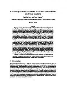
FIG. 1. Voronoi tessellation in a periodic box.
double contraction and 1 is the unit tensor. These equations have to be supplemented with the constitutive equations for ¯ of the viscous stress tensor, the traceless symmetric part ⌸ the trace ⌸ of the viscous stress tensor, and the heat flux Jq . They are
where 关 v兴 (t) is the average of the velocity field over cell . Therefore the Voronoi cells ‘‘follow’’ the flow field in a Lagrangian way. Here and in what follows, we denote with 关 ••• 兴 the spatial average of an arbitrary field over the Voronoi cell . After multiplying Eqs. 共1兲 with the characteristic function (r) of cell and using the mathematical tricks described in the Appendix, plus the gradient approximation also described there, it is straightforward to arrive at the following set of equations: ˙ ⫽ M
P˙ ⫽
¯ ⫽⫺2 ¯ “v, ⌸ ⌸⫽⫺ “•v, 1 Jq ⫽⫺ “T⫽ T 2 “ , T
共2兲
S˙ ⫽
A
Here, D is the dimension of physical space. In principle, the shear viscosity , the bulk viscosity , and the thermal conductivity might depend on the state of the fluid through ,s. The finite volume method consists of integrating Eqs. 共1兲 in a finite region of space 共or finite volume兲 in such a way that ordinary differential equations for the average fields over the finite regions emerge. We present a finite volume method that uses the Voronoi construction as a conceptually and mathematically elegant method for discretizing the continuum equations of hydrodynamics. The details are given in the Appendix where we use the smoothed characteristic function of the Voronoi cells introduced by Flekko” y et al. 关20兴 as a convenient mathematical tool 关25兴. Without the help of this smoothed characteristic function it is very difficult to figure out the effects of the Lagrangian moving grid in the final discrete equations. In the Appendix, we show how the method can be applied to a general balance equation, so we will simply quote in the present section the final results for the case of the set of equations 共1兲. The Voronoi tessellation is a way of partitioning space around a set of ‘‘cell centers’’ located at R by associating the region of space that is closer to that cell center than to any other center of the set. Each cell will have a volume V that depends parametrically on the positions of the cell centers. Figure 1 shows a two-dimensional 共2D兲 tessellation in a periodic box.
关 兴 ⫹ 关 兴 c • 共关 v兴 ⫺ 关 v兴 兲 , 2
关 兴 ⫹ 关 兴 关 v兴 ⫹ 关 v兴 c • 共关 v兴 ⫺ 关 v兴 兲 2 2
兺 ⍀ • 共关 P 兴 1⫹⌸ ⫹⌸ 1兲 , A
兺 R ⫹
共3兲
A
兺 R
兺 R ⫹
where the traceless symmetric part of the velocity gradient tensor is 1 1 “v⫽ 关 “v⫹ 共 “v兲 T 兴 ⫺ “•v. 2 D
共4兲
1 T
关 s 兴 ⫹ 关 s 兴 c • 共关 v兴 ⫺ 关 v兴 兲 2
2
兺 ⍀ • 关 Jq 兴 ⫹ T V G¯ :G¯ ⫹ T V D 2 . 共5兲
We have introduced in these equations the following quantities: total mass of cell M ⫽V 关 兴 , total momentum P ⫽V 关 g兴 , and total entropy S ⫽V 关 s 兴 , pressure and temperature of cell through 关 P 兴 ⫽ P eq( 关 兴 , 关 s 兴 ) and 关 T 兴 ⫽T eq( 关 兴 , 关 s 兴 ). Also, we introduced discrete versions of the constitutive equations 共2兲 through 2 ¯ ⫽⫺ 关 兴 G ¯, ⌸ V ⌸ ⫽⫺ 关 Jq 兴 ⫽⫺
关兴 D , V
关兴 2 T V
共6兲 1
兺 ⍀ T .
Here, the discrete versions of the symmetric part of the traceless velocity gradient tensor and the divergence of the velocity are defined
046115-3
¯ ␣ ⫽⫺ G
冋
1 2
1
兺 关 ⍀␣ v ⫹⍀ v␣ 兴 ⫺ D ␦ ␣ 兺 ⍀ •v D ⫽⫺
兺 ⍀ •v ,
册
, 共7兲
˜ OL MAR SERRANO AND PEP ESPAN
PHYSICAL REVIEW E 64 046115
The geometrical objects introduced in Eqs. 共5兲 are the area A between cells , and the 共half兲 normal surface vector 1 ⍀ ⫽ A e , 2
共8兲
where e ⫽(R ⫺R )/R is a unit vector normal to the face , . Finally, the vector c is a vector parallel to the face , as discussed in the Appendix. Despite its formidable aspect, Eqs. 共5兲 are quite natural if one looks at ⍀ as a sort of negative discrete gradient operator 关see Eq. 共A25兲 in the Appendix兴. In this way, every term in Eqs. 共1兲 and 共2兲 has its counterpart in Eqs. 共5兲 and 共6兲. One would expect that the convective terms of the continuum equations 共1兲 must disappear in a Lagrangian description. Rather, they are replaced by the terms involving c . These terms are associated with the rate of change of the extensive variables due to the change of shape of the cell as it moves, rather than to the main 共convective兲 motion of the cell. III.
GENERIC
MODEL OF FLUID PARTICLES
We could already use Eqs. 共5兲 for a numerical simulation of the continuum equations 共1兲. Because of the gradient approximation used in the derivation, these equations are accurate to first order in gradients. However, one can easily show that the energy at the discrete level is not strictly conserved by the above equations. In order to solve this problem and, most importantly, to introduce correct thermal fluctuations in the model, we cast in this section the previous equations within the GENERIC framework. Our point of view is that the Voronoi cells serve not only as a discretization tool for the hydrodynamic equations but also as a way of properly defining the concept of a fluid particle. In this paper, a fluid particle is understood as a thermodynamic subsystem of definite shape 共given by the Voronoi cell兲 that moves following the flow 关18兴. The state of the fluid is given by the set x ⫽ 兵 R ,P ,M ,S 其 where labels each of the M Voronoi fluid particles in the system and R is the position, P is the momentum, M is the mass, and S is the entropy of the th fluid particle. The volume V of the fluid particles is a function of the positions of the particles, i.e., V ⫽V (R1 , . . . ,RM ) and it is not an independent variable 关26兴. The energy and entropy functions are postulated to have the form E共 x 兲⫽
P2
兺 2M ⫹E共 M ,S ,V 兲 , S共 x 兲⫽
共9兲
兺 S ,
where V is an implicit function of the positions of the fluid particles, and E(M ,S ,V ) is the internal energy function. Because each fluid particle is understood as a thermodynamic subsystem, it has a well-defined thermodynamic fun-
damental equation. The fundamental equation relates the internal energy E of the fluid particle with its mass M , volume V , and entropy S , this is E ⫽E(M ,V ,S ). Regarding the dynamical invariants of the system, we require that the total mass M (x)⫽ 兺 M and total momentum P(x)⫽ 兺 P are the only dynamical invariants. Conservation of angular momentum would require the introduction of spin variables in this discrete model 关3兴. Now the basic question we pose is, what dynamical equations should we have for these discrete hydrodynamic variables x such that strict respect to the first and second laws of thermodynamics is guaranteed? In order to answer this question, we resort to the thermodynamically consistent GENERIC ¨ ttinger 关27兴. The formalism introduced by Grmela and O GENERIC dynamic equations are given by dx E S ⫽L ⫹M . dt x x
共10兲
The first term in the right-hand side corresponds to the reversible part of the dynamics and the second term corresponds to the irreversible part. The matrix L is antisymmetric whereas M is symmetric and positive semidefinite. Most important, the following degeneracy conditions should hold L
S ⫽0, x
M
E ⫽0. x
共11兲
These properties ensure that the energy is a dynamical invariant, E˙ ⫽0, and that the entropy is a nondecreasing function of time, S˙ ⭓0, as can be proved by a simple application of the chain rule and the equations of motion 共10兲. In the case that other dynamical invariants I(x) exist in the system 共as, for example, linear or angular momentum兲, then further conditions must be satisfied by L,M . In particular,
I E L ⫽0, x x
I S M ⫽0, x x
共12兲
which ensure that I˙ ⫽0. The deterministic equations 共10兲 are, actually, an approximation in which thermal fluctuations are neglected. If thermal fluctuations are not neglected, the dynamics is described by the following stochastic differential equations interpreted in Itoˆ sense 关27兴:
冋
dx⫽ L
册
E S ˜, ⫹M ⫹k B M dt⫹dx x x x
共13兲
to be compared with the deterministic equations 共10兲. The ˜ in Eq. 共13兲 is a linear combination of stochastic term dx independent increments of the Wiener process. It satisfies the Itoˆ rule ˜ dx ˜ T ⫽2k B M dt, dx
共14兲
˜ is an infinitesimal of order 1/2 关28兴. which means that dx Equation 共14兲 is a compact and formal statement of the fluctuation-dissipation theorem. Formally, the size of the
046115-4
THERMODYNAMICALLY CONSISTENT MESOSCOPIC . . .
PHYSICAL REVIEW E 64 046115
fluctuations is governed by the Boltzmann constant k B . If we take k B →0, the stochastic differential equation 共13兲 becomes the deterministic equations 共10兲. When formulating new models it might be convenient to ˜ directly instead of M. This ensures that M through specify dx Eq. 共14兲 automatically satisfies the symmetry and positive definite character. In order to guarantee that the total energy and dynamical invariants do not change in time, a strong ˜ holds, requirement on the form of dx
E ˜ ⫽0, dx x
I ˜ ⫽0. dx x
共15兲
E ⫽ x
冉 冊 ⫺
2
S ⫽ x
,
⫹
P˙
⫺ P ⫽
E ⫽ M E T ⫽ S
冏
兺
冏 冏
v
L
⫺
2
共20兲
,
⫹
T
,
共16兲
0
1␦
0
0
1
⫺1␦
⌳
⌬
⌫
0
⫺⌬
0
0
0
⫺⌫
0
0
, M ,S
共17兲
冊
.
共21兲
The first row of L ensures the equation of motion 共19兲. The first column is fixed by antisymmetry of L. Note that in order to have antisymmetry of L 共which, in turn, ensures energy conservation兲, it is necessary that ⌳T ⫽⫺⌳ . Performing the matrix multiplication in Eq. 共20兲, the reversible part of the dynamics takes the form ˙ ⫽v , R
,
S,V
P˙ ⫽
. M ,V
兺 ⫹
A e
兺
冋
P ⫺ P ⫹ 2
˙ ⫽⫺ M
We are now in position to formulate the dynamical equations.
S˙ ⫽⫺
兺
046115-5
兺
冉
⌳ v ⫺⌬
v2 2
冊 册
A c 共 P ⫺ P 兲 ⫹⌬ ⫹⌫ T , R
V P ⫺ P A ⫹ P ⫽ A e c 共 P ⫺ P 兲 . R ⫽ 2 ⫽ R 共18兲
兺
v2
0
We can develop the pressure term in E/ x by using Eqs. 共A32兲 and 共A34兲 in the Appendix,
兺
V
兺␥ R␥ P ␥
where the block L has the structure
0
P , M
E V
⫽
˙ M
where we have introduced the velocity v , pressure P , chemical potential per unit mass , and temperature T according to the usual definitions, v ⫽
冉 冊 ⫺
˙ R
L ⫽
T
共19兲
The simplest nontrivial reversible part that produces the above equation has the following form:
0
v
v2
˙ ⫽v . R
S˙
V␥ P R ␥
兺␥
In this section we consider the reversible part of the dynamics for the fluid particle model. The matrix L is made of M ⫻M blocks L of size 8⫻8. The antisymmetry of L translates into L ⫽⫺L . We have first strong requirements for the form of L. We wish that the reversible part of the dynamics produces the following equations of motion for the positions:
冉冊 冉冊 冉
The geometrical meaning of Eq. 共15兲 is clear. The random ˜ on the state x are orthogonal to the kicks produced by dx gradients of E,I. These gradients are perpendicular vectors 共strictly speaking they are one forms兲 to the hypersurface E(x)⫽E 0 , I(x)⫽I 0 . Therefore the kicks let the state x always within the hypersurface of dynamical invariants. For future reference, the derivatives with respect to the state variables of the energy and entropy are given by ⫺
A. Reversible dynamics
兺 ⌬ v ,
兺 ⌫ v .
共22兲
˜ OL MAR SERRANO AND PEP ESPAN
PHYSICAL REVIEW E 64 046115
What forms for ⌳ , ⌬ , and ⌫ should we use in order to consider Eqs. 共22兲 as a discrete version of inviscid hydrodynamics? In what follows we will propose forms for these quantities in such a way that Eqs. 共22兲 and 共5兲 共with zero transport coefficients兲 coincide as much as possible. The vectors ⌬ and ⌫ are easily identified by comparing the mass and entropy equations in Eqs. 共5兲 and 共22兲. The matrix ⌳ is obtained by inspection from the comparison between the momentum equation in Eqs. 共5兲 and 共22兲. Our proposals are therefore, ⌬ ⫽
A ⫹ c ⫺ ␦ R 2
兺 R
A
⫹ c , 2
A s ⫹s c ⫺ ␦ R 2
兺 R
A
s ⫹s c , 2
⌫ ⫽
⌳ ⫽⫺
冋
v ⫹v A ⫹ v ⫹v c ⫺c R 2 2 2
⫹ ␦
冋
册
⫹ v ⫹v v ⫹v . c ⫺c 2 2 2
A
兺 R
Note that ⌳T ⫽⫺⌳ ⫽⫺⌳ and therefore the antisymmetry of L is ensured. Note also that 兺 ⌫ ⫽0 and therefore the degeneracy condition L S/ x⫽0 is satisfied. By substitution of these forms 共23兲 into Eq. 共22兲 one obtains the proposed GENERIC equations for the reversible part of the evolution of R ,P ,M ,S , that is,
⫺
P˙ ⫽
兺
⫻c • 共 v ⫺v 兲 ⫹ ⫻共 ⫺ 兲⫺
˙ ⫽ M
S˙ ⫽
兺
A
In this section we consider the irreversible part of the ˜ dynamics M S/ x. We will postulate the random terms dx for the discrete equations and will construct, through the fluctuation-dissipation theorem 共14兲, the matrix M and the irreversible part of the dynamics. If we guess correctly the random terms, the resulting discrete equations should consistently produce the correct dissipative part of the dynamics. According to Landau and Lifshitz, thermal fluctuations are introduced into the continuum equations of hydrodynamics through the divergence of a random stress tensor and a random heat flux 关16,29兴. In our discrete case, the noise term in the equation of motion 共13兲 is postulated to have the form ˜ T →(0,dP ˜ ,0,dS ˜ ), where the random terms dP ˜ ,dS ˜ are dx the discrete divergences of a random flux, i.e.,
冋
册
兺 R
⫹ c • 共 v ⫺v 兲 , 2
A
s ⫹s c • 共 v ⫺v 兲 . 2
兺 R
兺 ⍀ •d ˜ , 共26兲
A ⫹ v ⫹v R 2 2
兺 R c 共 P ⫺ P 兲 ⫺
共25兲
This term is strongly reminiscent of the Gibbs-Duhem relation that, in differential form, is d P⫺ d ⫺sdT⫽0. For this reason, we expect that this term 共25兲, although not exactly zero, will be very small. Therefore Eqs. 共24兲 can be considered as a proper discretization of the continuum equations of inviscid hydrodynamics. Total mass, momentum, and energy are conserved exactly and the total entropy does not change in time due to this reversible motion.
˜ ⫽ dP
s ⫹s 共 T ⫺T 兲 , 2
A
册
s ⫹s 共 T ⫺T 兲 . 2
˙ ⫽v , R P ⫺ P ⫹ A e 2
⫹ 共 ⫺ 兲 2
B. Irreversible dynamics
共23兲
册
冋
A
兺 R c 共 P ⫺ P 兲 ⫺
˜ ⫽ dS
⫹ 2
1 T
1
兺 ⍀ •dJ˜q ⫺ T d ˜ : 兺 ⍀ vT .
˜ and random heat flux dJ ˜ q are deThe random stress d fined by
共24兲 ˜ ⫽a dWS ⫹b d
1 tr关 dW 兴 , D 共27兲
˜ q ⫽c dV . dJ The coefficients a ,b ,c are given by
Here, v ⫽P /M , ⫽M /V , and s ⫽S /V . These GENERIC equations 共24兲 for the reversible part of the dynamics are identical to the finite volume discretization of the continuum equations of inviscid hydrodynamics, Eqs. 共5兲 with zero transport coefficients, except for the following term in the momentum equation: 046115-6
冉
a ⫽ 4k B T
冉
V
b ⫽ 2Dk B T
冊
V
1/2
,
冊
1/2
,
THERMODYNAMICALLY CONSISTENT MESOSCOPIC . . .
冉
c ⫽T 2k B
V
冊
PHYSICAL REVIEW E 64 046115
冉
1/2
.
共28兲
Here, D is the physical dimension of space, is the shear viscosity, is the bulk viscosity, and is the thermal conductivity. These transport coefficient might depend in general on the thermodynamic state of the fluid particle . The particular form of the coefficients in Eq. 共28兲 might appear somehow arbitrary. Actually, it is only after writing up the final discrete equations and comparing them with the finite volume equations 共5兲 that we could extract the particular functional form of these coefficients. Finally, note that the noise amplitudes scale as the inverse square root of the volume, impliying that for very large cells the noise can be neglected. The traceless symmetric random matrix dWS is given by 1 1 dWS ⫽ 关 dW ⫹dWT 兴 ⫺ tr关 dW 兴 1. 2 D
共29兲
dW is a matrix of independent Wiener increments. The vector dV is also a vector of independent Wiener increments. They satisfy the Itoˆ rules of stochastic calculus dWii ⬘ dWj j ⬘ ⫽ ␦ ␦ i j ␦ i ⬘ j ⬘ dt, dVi dVj ⫽ ␦ ␦ i j dt,
共30兲
dVi dWj j ⬘ ⫽0,
T dS 兩 irr⫽ 1⫺ ⫹
兺
共31兲
兺 dP˜ ⫽0, and therefore Eqs. 共15兲 are satisfied. This means that the postulated noise terms conserve momentum and energy exactly. It is now a matter of algebra to construct the dyadic ˜ dx ˜ T and from Eq. 共14兲 extract the matrix M. The procedx dure is rather cumbersome but standard. Once M is constructed, the terms M • S/ x in the equation of motion 共10兲 can be written up. By assuming that the transport coefficients do not depend on the entropy density 共but they might depend on the mass density兲, the resulting equations of motion are dP 兩 irr⫽
兺 ⍀ • 共 ⌸ ⫹⌸ 1兲 dt⫹dP˜ ,
共32兲
冊冋
册
2 ¯ :G ¯ ⫹ D 2 dt G V V k
冊
册兺
兺 ⍀ •Jq dt⫺ T CB 兺 ⍀2 V T 2 dt
⫺k B T
冋冉
D 2 ⫹D⫺2 2 ⫹ 2D V V
⍀2 M
dt
˜ . ⫹T dS In these equations, we have introduced the same quantities as in Eq. 共7兲. The heat flux Jq is defined by Jq ⫽⫺T 2
V
1
兺 ⍀ T
冉
1⫺
冊
kB . C
共33兲
Finally, the heat capacity at constant volume of fluid particle is defined by C ⫽T
冉 冊
⫺1
T s
共34兲
.
We observe that, quite remarkably, the above equations are in the limit k B →0 identical to the irreversible part of the particular finite volume discretization of the continuum hydrodynamic equations presented in Sec. II. We have therefore shown that these equations 共32兲 are a proper discretization of the irreversible part of hydrodynamics with thermal noise included consistently. By collecting the reversible part in Eq. 共24兲 and the irreversible part in Eq. 共32兲, the final equations of motion for the discrete hydrodynamic variables can be finally written.
where Latin indices denote tensorial components. Note that ˜ ,dS ˜ in Eq. 共26兲 satisfy the postulated forms for dP ˜ ⫹T dS ˜ ⫽0, v •dP
kB C
IV. SIMULATION RESULTS
We have implemented a code in which Eqs. 共24兲 together with the irreversible terms 共32兲 are simulated. A 2D box with periodic boundary conditions has been tessellated according to the Voronoi construction. Because no forcing boundary conditions are considered in this paper, the typical experiments consist of a decay of an initial state towards the equilibrium state. A. Ideal gas
The fluid has been assumed to be an ideal gas, for which the fundamental equation is given by E共 N,V,S 兲 ⫽
冉冊 再冉
DNh 2 N 4m0 V
2/D
exp
2 S D⫹2 ⫺ D Nk B 2
冊冎
. 共35兲
Here, N is the number of molecules 共so Nm 0 is the mass of the system and m 0 is the mass of a molecule兲, h is Planck’s constant, and D is the number of space dimensions. The equations of state give the temperature, chemical potential per particle, and the pressure as
046115-7
˜ OL MAR SERRANO AND PEP ESPAN
T⫽
冉 冊 E S
⫽ N,V
冉 冊 冉 冉 冊
E *⫽ N
PHYSICAL REVIEW E 64 046115
2 E, DNk B
˜S ⫽
冊
2⫹D 1 2S ⫽E , ⫺ D N DN 2 k B V,S
E P⫽⫺ V
˜V ⫽
N ⫽ k B T. V N,S
冉 冊 E T
⫽ N,V
D Nk B . 2
共37兲
It must be remarked that we assume that each cell has associated with it a fundamental equation 共35兲 and therefore the intensive parameters 共36兲. The N in Eq. 共35兲 thus refers to the number of molecules in a given cell. These cell intensive parameters are the quantities that enter the equations of motion of the system. We are not assuming that the system considered as a whole will behave as an ideal gas. Even though physically we expect that this is the case we must check that our simulations do satisfy this requirement 共see Sec. IV G兲.
˜ ⫽ M
The four basic units selected are the mass unit m u ⫽N micm 0 , the entropy unit S u ⫽N mick B , the length unit L u ⫽N 1/D mic, and the temperature unit T u ⫽T e . Any other unit is derived from these ones. Here, m 0 is the mass of one molecule 共or atom兲 of the ideal gas, is the typical distance between molecules at room conditions, and T e ⫽273 K is the room temperature. N mic is an arbitrary number. If we choose N mic to be equal to the total number of molecules in the sample being simulated, then the total mass of the system is 1 in these units. If the system is at room temperature, then T⫽1 in these units, the mass density is 1 and the box size is also 1. We introduce these units that refer essentially to the global quantities of the sample being simulated. We could select units referred to the Voronoi cell in such a way that the typical mass of a cell would take value 1. This would imply that simulations with different number of cells would correspond to samples of different sizes rather than to the same sample with different resolution. We introduce the following reduced quantities:
˜P ⫽
˜⫽
k B N micT e
.
共39兲
which is the fraction of the molecules or atoms of the whole sample that are in the cell . With these reduced units, one can write the thermodynamic relations 共35兲 and 共36兲 in dimensionless form, ˜E共 M ˜ ,S ˜ ,V ˜ 兲 ⫽M ˜ ˜T 共 M ˜ ,S ˜ ,V ˜ 兲, ˜T 共 M ˜ ,S ˜ ,V ˜ 兲⫽
1 ␣
˜ M exp ˜V
再 冎
˜S ⫺2 , ˜ M
˜ ˜T M ˜P ⫽ , ˜V
共40兲
˜ ⫽M ˜. C The dimensionless chemical potential per unit mass is given by ˜⫽
冉 冊 冉 ˜E ˜ M
˜ ⫽E
˜V ,S ˜
冊
˜S 2 ⫺ 2 . ˜ ˜ M M
共41兲
In Eqs. 共40兲, we have introduced the dimensionless constant ␣ that depends only on microscopic parameters through
冉冊
␣⫽ ⌳
2
⫽
22 m 0k BT e h2
,
共42兲
where ⌳ is the thermal wavelength. With these dimensionless quantities, the equations of motion are identical to Eqs. 共24兲 and 共32兲 with a tilde on every variable.
T , Te
PL 2u
L 2u
m N m 0 N ⫽ ⫽ , m u N micm 0 N mic
B. Reduced units
˜T ⫽
V
If N is the number of molecules in the mesoscopic cell 共we have 兺 M⫽1 N ⫽N mic) the dimensionless mass of cell is
The specific heat at constant volume is C⫽
E , k B N micT e
˜E ⫽
共36兲
S , k B N mic
C. Parameters used in the simulations
,
, k B N micT e
共38兲
We want to simulate a sample of argon, assumed to be an ideal gas, whose molecules have a mass m 0 ⫽6.6325⫻10⫺26 kg. The system is assumed to be at room temperature. The number of molecules in the sample is N mic⫽4⫻104 . We use M ⫽400 mesoscopic Voronoi cells to discretize the 2D box, which lead to typically 100 argon atoms in each cell. The typical distance between molecules
046115-8
THERMODYNAMICALLY CONSISTENT MESOSCOPIC . . .
PHYSICAL REVIEW E 64 046115
in an ideal gas at room temperature and pressure in three dimensions is ⫽3⫻10⫺9 m. If in two dimensions we want to keep this typical distance, then the linear dimensions of 1/2 3⫻10⫺9 m⫽6.67⫻10⫺7 our simulation box should be N mic m. The constant ␣ in Eq. 共42兲 takes the value ␣ ⫽3.987 138 93⫻104 . The dimensionless shear and bulk viscosities and thermal conductivity are taken as ˜ ⫽˜ ⫽ ˜ ⫽0.01. D. Deterministic simulations
As a first test of the algorithm, we have conducted simulations in which the terms proportional to k B in Eqs. 共32兲 have been neglected. This results in deterministic equations that should reproduce the results of continuum hydrodynamics. The time integrator scheme that we have used in this deterministic case is a Runge-Kutta method of fourth order. We have also devised a generalization of the time reversible velocity-Verlet algorithm 共that conserves total energy兲. This generalization has been constructed as an application of the Tuckerman formalism, which makes extensive use of the Trotter expansion 关30兴. The Runge-Kutta method has fourth order precision in front of the second order precision of the generalized velocity Verlet. In spite of the longer CPU time required by the Runge-Kutta method, it can use longer time steps to get the same precision. Most of the results presented below are obtained with the Runge-Kutta method with a time step d˜t ⫽0.01. According to the results of the linearized hydrodynamic equations, the evolution of the Fourier transforms of the perturbation from equilibrium for the mass (k,t) and momentum g(k,t) density fields have the form c 共 k,t 兲 ⫽⫺i exp兵 ⫺⌫k 2 t 其 sin共 ckt 兲 kˆ•g共 k,0兲 ,
共43兲 g共 k,t 兲 ⫽exp兵 ⫺⌫k 2 t 其 cos共 ckt 兲 kˆkˆ•g共 k,0兲 ⫹exp兵 ⫺ k 2 t 其 ⫻ 关 1⫺kˆkˆ兴 •g共 k,0兲 ,
FIG. 3. Temporal evolution of the total entropy of the system for the transverse perturbation experiment. It is a strictly increasing function of time.
sound speed, ⌫ is the sound absorption coefficient, and ⫽ / is the kinematic shear viscosity. If the initial perturbations fields are
共 r,0兲 ⫽0, g共 r,0兲 ⫽exp兵 ik0 •r其 g0 , then, in Fourier space, we will have
共 k,0兲 ⫽0, 共 2 兲D g共 k,0兲 ⫽ 关 ␦ 共 k⫺k0 兲 ⫹ ␦ 共 k⫹k0 兲兴 g0 , 2
共45兲
where g0 ⫽ v0 , with v0 ⫽( v 0 ,0,0). Including these initial conditions in Eqs. 共43兲 we see that the non vanishing results are for the k⫽⫾k0 . Selecting the longitudinal kL ⫽(k 0 ,0,0) and transverse kT ⫽(0,k 0 ,0) wave vectors, it is possible to disentangle the effects of diffusion of vorticity and the propagation of sound. In the longitudinal case we have
where kˆ is the unit vector along the wave vector, c is the c 共 kL ,t 兲 ⫽⫺i exp兵 ⫺⌫k 20 t 其 sin共 ck 0 t 兲
FIG. 2. Dots are for the transverse momentum field in Fourier space as a function of time. The theoretical fit in continuum line 共invisible under the dots兲 corresponds to ˜ ⫽0.009 680 共the input value is ˜ ⫽0.01). The resolution is for a typical number of 20 cells per box length L.
共44兲
共 2 兲D L kˆ •v0 , 2
共46兲
FIG. 4. Temporal evolution of the individual pressures of 20 particles for the transverse perturbation experiment. At equilibrium all the particles have the same pressure. Solid line is for particle 1.
046115-9
˜ OL MAR SERRANO AND PEP ESPAN
PHYSICAL REVIEW E 64 046115
FIG. 5. Temporal evolution of the individual temperatures of 20 particles for the transverse perturbation experiment. At equilibrium all the particles have the same temperature. Solid line is for particle 1.
g共 kL ,t 兲 ⫽exp兵 ⫺⌫k 20 t 其 cos共 ck 0 t 兲
共 2 兲D L L kˆ kˆ •v0 . 2
E. Transverse wave
In the transversal case we have
共 kT ,t 兲 ⫽0, 共47兲 g共 kT ,t 兲 ⫽exp兵 ⫺ k 20 t 其
FIG. 7. Temporal evolution of the total entropy of the system for the longitudinal perturbation experiment. Despite slight oscillations due to the wave character of the perturbation, the entropy is a strictly increasing function of time.
共 2 兲D v0 . 2
In the simulations, the reduced temperature is initially set ˜ to T ⫽1 and the reduced density to ˜ ⫽1. The initial value of the velocities of every cell is given by a longitudinal or transversal plane wave with a velocity amplitude ˜v 0 ⫽0.01, and a ˜ . We measure the Fourier compowave vector ˜k 0 ⫽(2 )/L nents of the mass and momentum density fields and fit its evolution with the theoretical predictions 共46兲 and 共47兲. From this fit, we measure the kinematic viscosity, the sound speed, and the sound absorption coefficient.
FIG. 6. In dots, the imaginary part of the longitudinal density field in Fourier space as a function of time. The continuum line is the theoretical expression with ˜⌫ ⫽0.012 27 and ˜c ⫽1.3937. The resolution is for a typical number of 20 cells per box length L.
In Fig. 2 we plot the transverse momentum field in Fourier space as a function of time. We get an excellent agreement with the theoretical exponential decay predicted by Eq. 共47兲. For the case of the transverse perturbation, we have recorded the total energy evolution as a function of time and have checked that it is a conserved quantity with an error that is 108 smaller than the total value. The total entropy evolution is reflected in Fig. 3. It is clearly a nondecreasing function of time. We have also monitored the pressures in Fig. 4 and the temperatures in Fig. 5 of a subset of 20 particles as the system approaches equilibrium. We can appreciate that the system reaches the equilibrium when all the particles take the same values for these intensive variables. F. Longitudinal wave
For the longitudinal experiment, we plot in Fig. 6 the imaginary part of the longitudinal density field in Fourier space as a function of time along with the theoretical prediction 共46兲. In this simulation, the total energy is conserved with an error that is 108 times smaller than the total value. The total
FIG. 8. Temporal evolution of the individual pressures of 20 particles of the total system for the longitudinal perturbation experiment. Solid line is for particle 1.
046115-10
THERMODYNAMICALLY CONSISTENT MESOSCOPIC . . .
FIG. 9. Temporal evolution of the individual temperatures of 20 particles of the total system for the longitudinal perturbation experiment. Solid line is for particle 1.
entropy is again a strictly nondecreasing function of time, see Fig. 7. We again plot the time evolution of the pressures in Fig. 8 and thermodynamic temperatures in Fig. 9 for a subset of 20 particles. The equilibrium state is established when all the particles take identical values for these variables. It is interesting to make a systematic study of the transport coefficients in terms of the resolution. We define the resolution as the typical number of cells per unit length (M 1/D /L). In Fig. 10 we plot the kinematic viscosity measured in simulations of decaying transverse waves for different number of cells in the box. The input value is given by the solid line. As we increase the resolution we obtain an excellent agreement between measured and input values. The sound speed for the ideal gas is given by
PHYSICAL REVIEW E 64 046115
FIG. 11. The sound velocity c measured through the oscillation of the imaginary part of the density field in Fourier space for dif˜ in conferent resolutions (M 1/D /L). The predicted value is ˜c ⫽ 冑2T tinuum line.
an accuracy of 2% of the input viscosity and 1% of the input sound speed. These results provide a very satisfactory test of our deterministic code. G. Proof of the local equilibrium assumption
˜ . In Fig. 11 we plot which in reduced units becomes ˜c ⫽ 冑2T the measured sound speed and the input value. Our simulations results agree very well with the linear solutions of the hydrodynamic equations and show that a resolution of typically 25 particles per box length L provides
A very interesting observation about the previous shear and sound wave simulations is that the time evolution of the entropy in Figs. 3 and 7 is such that the final values of the total entropy in each simulation are exactly the same. The initial value of the entropy is fixed by the initial conditions. Because the only difference in both initial conditions is in the velocity variable, and the entropy is independent of the velocity, the initial total entropy of both simulations are the same. At the same time, both simulations have initial conditions such that the global conserved quantities 共mass, volume, energy兲 are exactly the same. Therefore the final value of the total entropy is seen to depend only on the global conserved quantities and not on the way the system evolves in order to reach the equilibrium state. This is, of course, the requirement of equilibrium thermodynamics. In order to better clarify this point, we plot in Fig. 12 the time evolution of the total entropy for the decay of a shear wave in two simulations differing only on the value of the transport coeffi-
FIG. 10. Dots correspond to the kinematic viscosity ˜ measured through the exponential decay of the momentum field in Fourier space for different resolutions M 1/D /L). The solid line is the input kinematic viscosity.
FIG. 12. Total entropy S⫽ 兺 S as a function of time. Circles are for shear, bulk, and thermal conductivity equal to 0.01, squares for 0.03. Solid line is the total entropy computed from the thermodynamic equation of the ideal gas.
c⫽
冑 冉 冊 ⫺V
P . V s
共48兲
046115-11
˜ OL MAR SERRANO AND PEP ESPAN
PHYSICAL REVIEW E 64 046115
FIG. 13. Instantaneous evolution of the total energy in time. The dotted line corresponds to the model without the Gibbs-Duhem term 共25兲 and the continuum line to the GENERIC model, for a time step ⌬t⫽0.005.
cients. We observe that both simulations start at the same value 共because the initial conditions are identical兲 and that they approach to the same value of the entropy. The horizontal line is the value of the entropy computed from S(M 0 ,V 0 ,E 0 ), where M 0 ,V 0 ,E 0 are the total mass, total volume, and total energy of the system. The function S(M 0 ,V 0 ,E 0 ) is the inverse function of Eq. 共35兲. The fact that the total entropy increases to the value predicted by thermodynamics is a nontrivial result. Physically, we certainly expect that the total entropy at equilibrium is a function of state depending only on the extensive variables of the whole system. That our simulation technique obeys this physical requirement is a very pleasant outcome, which was not entirely expected beforehand. Another way to look at this issue is as follows. Even though in the technique we only specify the thermodynamic behavior of each cell 共i.e., each subsystem兲, the postulated dynamics is such that the final equilibrium thermodynamic behavior of the whole system is exactly the same as that of its subsystems. In other words, our technique respects the local equilibrium assumption. Once we have checked this property, we have a route to specify the internal energy function of each cell if we know the fundamental equation of the whole system. Note that the final value of the entropy in Fig. 12 does not depend on the actual values of the transport coefficients. Higher the dissipation, faster is the approach to the same equilibrium state. If the dissipation decreases, the equilibration time increases. In the limit of zero dissipation, the entropy is a constant of motion, equal to the value at the initial time, and the system will never reach the equilibrium state predicted by thermodynamics. The Euler equations for an inviscid fluid are clearly inconsistent with the principles of equilibrium thermodynamics. A dissipation is required, no matter how small, in order to drive the system towards the equilibrium state predicted by thermodynamics. H. Decay of temperature inhomogeneities
In the previous sound and shear wave simulations, the variation of the intensive parameters is very small 共see Figs. 4 and 5, and 8 and 9兲. We have conducted another simulation in which the cells are initially at different temperatures and
FIG. 14. The conservation of energy as a function of time step, for the model without the Gibbs-Duhem term 共triangles兲 and for the full model 共circles兲. The logarithm is in base 10.
velocities, depending on their y position. The upper half cells are at temperature T⫽1 while the lower half are at temperature T⫽2. An initial shear wave provides the initial velocities of the particles. Rather than focusing on measurements of thermal conductivities, we are interested in quantifying the actual size of the Gibbs-Duhem term 共25兲. Note that this term is very small in the previous simulations because of the very small differences between the intensive parameters of the cells. For this reason, we consider here the situation in which potentially this term is larger. We recall that this term is responsible for the exact energy conservation of the GENERIC algorithm. For this reason, we compare two simulations in the two-temperature configuration in which the Gibbs-Duhem term 共25兲 is included or removed in the momentum equation. In Fig. 13, we plot the instantaneous evolution of the total energy about the initial value for the two models. That is, we plot ⌬E 共 t 兲 ⫽
E 共 t 兲 ⫺E 共 0 兲 E共 0 兲
共49兲
We observe a cooling effect in the model without the Gibbs-Duhem term due to the nonconservation of the energy. There is still a slight increase in the energy in the GENERIC model that is due to numerical integration errors. In order to quantify these errors as a function of the timestep ⌬t, we measure the quantity
⌬Eˆ 共 ⌬t 兲 ⫽
1 N
N
兺 k⫽1
冏
冏
E 共 k⌬t 兲 ⫺E 共 0 兲 . E共 0 兲
共50兲
A fixed total time of N⌬t⫽4 is chosen. In Fig. 14, we plot the dependence of ⌬Eˆ on ⌬t for the two models. The result is very revealing. For the GENERIC model, we achieve any desired improvement of the energy conservation as the time step tends to zero. For the model without the Gibbs-Duhem term, the energy conservation is not improved as the time step goes to zero, but rather it converges to a typical value of 10⫺6 for this particular simulation.
046115-12
THERMODYNAMICALLY CONSISTENT MESOSCOPIC . . .
FIG. 15. How to tailor a solid horizontal flat wall boundary with the Voronoi tessellation by using pair boundary points.
PHYSICAL REVIEW E 64 046115
FIG. 17. Mass equilibrium distribution function. Dots correspond to simulation results. The continuum line is the theoretical prediction according to the Einstein distribution function.
Note that the Gibbs-Duhem energy producing term is very small, as concluded from these plots. Actually, if large time steps are used, the numerical error in the full model is already as large as this term.
of both centers of each boundary pair to be prescribed. We expect to present results on the implementation of boundary conditions in the near future.
I. Boundary conditions
J. Fluctuations included
In this paper we only consider systems with periodic boundary conditions. However, it is rather easy to implement other boundary conditions on given solid boundaries. The first issue to resolve is how to tessellate the space in order to conform with the prescribed geometric boundaries. In Fig. 15 we show that by collecting boundary pairs of fixed cell centers, one can easily construct flat walls. Other geometric shapes can be tailored in a similar way. Every pair has a center ‘‘within’’ the fluid domain and a center ‘‘outside’’ the fluid domain. If the boundary conditions are of the Neumann type, one needs to specify fluxes at the boundaries. In this case, for every ‘‘within’’ cell center of the pair, one has that the interaction with the ‘‘outside’’ cell center is fixed in terms of the prescribed flux. In the case that Dirichlet boundary conditions must be satisfied 共like in a no-slip boundary condition兲, one enforces the value of the hydrodynamic fields
We have also performed a test of the full algorithm in which thermal fluctuations are included. The evolution equations are now the stochastic differential equations 共24兲 and 共32兲. We modify consequently the integrator scheme. We choose an Euler algorithm that conserves total momentum and energy with a time step d˜t ⫽0.000 001. The initial state is set as follows. From a random distribution of cell positions in the box, we construct the Voronoi cells. Every cell has a given volume and we select its initial mass in order to have a constant density ˜ ⫽1. The initial velocity of the cells is zero. The initial entropy of each cell is selected in such a way that the temperature of every cell is ˜T ⫽1. Note that this initial state although close to equilibrium is not a typical equilibrium state. We let the system evolve and after a decay time we measure the equilibrium momentum, mass, and volume distribution functions for a single cell. The results are presented in Figs. 16,17,18,19, where the simulation results are presented along with the theoretical prediction obtained from the Einstein distribution
FIG. 16. Equilibrium momentum distribution function. Dots correspond to the simulation results and the continuum line corresponds to the theoretical prediction obtained from the Einstein distribution function. The dot-dashed line correspond to the best Gaussian and shows that the momentum distribution function is not strictly Gaussian. This is due to the fact that the mass of the fluid particles is allowed to evolve.
FIG. 18. Volume equilibrium distribution function. Dots correspond to simulation results. The continuum line is the theoretical prediction according to the Einstein distribution function.
046115-13
˜ OL MAR SERRANO AND PEP ESPAN
PHYSICAL REVIEW E 64 046115
S关 t 兴 ⫽
冕
S 共 x 兲 共 x,t 兲 dx⫺k B
冕
共 x,t 兲 ln 共 x,t 兲 dx,
共52兲
which is a functional of the time-dependent probability distribution function (x,t), it is possible to prove by using the Fokker-Planck equation corresponding to Eqs. 共13兲 that t S关 t 兴 ⭓0. In other words, the entropy functional plays the role of a Lyapunov function. V. SUMMARY AND CONCLUSIONS FIG. 19. Density equilibrium distribution function. Dots correspond to simulation results. The continuum line is the theoretical value obtained from the Einstein distribution function.
function 共51兲. The agreement is quite remarkable and provides confidence on the coding of the model. The Einstein distribution function 共in the presence of dynamical invariants 关31兴兲 is given by
eq共 x 兲 ⫽
␦ „E 共 x 兲 ⫺E 0 …␦ „I 共 x 兲 ⫺I 0 … ⍀ 共 E 0 ,I 0 兲
exp兵 k B⫺1 S 共 x 兲 其 , 共51兲
where ⍀(E 0 ,I 0 ) is the normalization. It can be shown that the Fokker-Planck equation that is mathematically equivalent to the stochastic equations 共13兲 has as equilibrium solution the Einstein distribution function. The details of the derivation of the theoretical predictions for the single cell distribution functions from the M-particle Einstein distribution function 共51兲 will be given in a separate publication 关32兴. An interesting observation is the fact that in the stochastic simulation the total entropy of the system is a fluctuating quantity that is not strictly an increasing function of time. In an equilibrium situation it fluctuates around a constant value as shown in Fig. 20. It must be clearly understood that this does not contradict the second law of thermodynamics, which is a macroscopic law. Note that the fluctuations in the entropy are of the order of the Boltzmann constant, which is negligible in macroscopic terms. Actually, if one considers the entropy functional
FIG. 20. Time evolution of the total entropy in an equilibrium state for a system with thermal fluctuations.
In this paper we have considered a Lagrange finite volume model for simulating hydrodynamics in the presence of thermal fluctuations. We have paid special attention to the thermodynamic consistency of the model by casting it within the GENERIC framework. The obtained equations conserve mass, momentum, energy, and volume and the entropy is a strictly increasing function of time in the absence of fluctuations. Thermal fluctuations are consistently included, which lead to the strict increase of the entropy functional and to the correct Einstein distribution function. The size of the thermal fluctuations is given by the typical size of the volumes of the particles, arguably scaling like the square root of this volume. The need of incorporating thermal fluctuations in a particular system will be determined by the external length scales that need to be resolved. For example, if submicron colloidal particles are considered, we need to resolve the size of the colloidal particle with fluid particles of size, say, an order of magnitude or two smaller than the diameter of the colloidal particle. For these small volumes, fluctuations are important and lead to the Brownian motion of the particle. A ping-pong ball, on the other hand, requires fluid particles much larger, for which thermal fluctuations are negligible. Of course, one could use a very large number of small fluid particles to deal with the ping-pong ball, but in this case the 共large兲 thermal fluctuations on each fluid particle average out among the 共large兲 number of fluid particles. The original formulations of dissipative particle dynamics lack this effect of switching off thermal fluctuations depending on the size of the fluid particles. This is due to the fact that early formulations did not include the volume and/or the mass of the particles as a relevant dynamical variable. The main difference of our approach from that of Flekko” y et al. 关20兴 is the different form of the actual dissipative forces between the fluid particles. As a consequence, the explicit form of the thermal fluctuations is also different. In our case, the forces are given in terms of discrete versions of the gradient of the stress tensor, which are given, in turn, by discrete versions of the velocity gradients. Therefore, the viscous forces between a pair of fluid particles depend not only on the velocities of the pair but also on the velocity of the neighbors of both particles. Therefore, the amount of information about the fluid state around the pair of cells is quite large. In Ref. 关20兴 the forces are given directly in terms of velocity differences between the particles of the pair. Although it can be shown that the proposed equations in Ref. 关20兴 can be understood as a discretization of Navier-Stokes
046115-14
THERMODYNAMICALLY CONSISTENT MESOSCOPIC . . .
关33兴, and that the resulting equations of Ref. 关20兴 have actually the GENERIC structure, it remains to be investigated to what degree both algorithms compare in terms of the number of particles needed to obtain a good resolution of given flows. The notion of Voronoi cells allows for a very clear statement of the problem of coupling continuum equations and molecular dynamics, which is important when the continuum description breaks down due to complex molecular details in certain regions as the contact line of two fluids and a solid, or the tip singularity in dynamic fracture. A promising approach has been taken in Ref. 关34兴 in that direction.
PHYSICAL REVIEW E 64 046115
Some useful properties of the smoothed characteristic function will be needed later. First, due to the Gaussian form of ⌬(r), “⌬ 共 r 兲 ⫽⫺
兺
,
lim 共 r兲 ⫽
共 r兲关 1⫺ 共 r兲兴 ⫽
共A2兲
where (x) is the Heaviside step function. The Voronoi characteristic function 共A2兲 takes the value 1 if r is nearer to ” . Note that the characterR than to any other R with ⫽ istic function produces a covering of all space 共i.e., a partition of unity兲, that is,
兺 共 r兲 ⫽1.
共A3兲
We introduce the volume of the Voronoi cell through V ⫽
冕
VT
dr 共 r兲 ,
1 共 r兲 ⫽ 2 r
共A1兲
⌬ 共 兩 r⫺R 兩 兲
兿 共 兩 r⫺R兩 ⫺ 兩 r⫺R兩 兲 ,
where V T is the total volume.
共A7兲
兺
” ⫽
共 r兲 共 r兲 ,
共A8兲
共A9兲
We illustrate how the smooth Voronoi characteristic function can be used for deriving a finite volume discretization of a balance equation for a field (r,t),
t 共 r,t 兲 ⫽⫺“•J共 r,t 兲 ,
共A10兲
where J(r,t) is an appropriate current density, which will depend, through a constitutive equation on (r,t) itself. First, we introduce the cell average 关 兴 (t) over the Voronoi cell of the field (r,t) 关 兴 共 t 兲 ⫽
1 V
冕
dr 共 r,t 兲 共 r兲 .
共A11兲
We will refer to 关 兴 (t) as a cell variable. The cell variable is an approximation for the value of the field at the discrete points given by the cell centers. In principle, the Voronoi cell centers are allowed to move in an arbitrary way, that is, R (t) are prescribed functions of time. The time derivative of the cell averages is given by d V˙ 1 关 兴 共 t 兲 ⫽⫺ 关 兴 共 t 兲 ⫹ dt V V
共A4兲
⫹ 共A5兲
兺 共 r兲 共 r兲共 R ⫺R 兲 .
1. Balance equations
which satisfies the closure condition
兺 V ⫽V T ,
兺 共 r兲共 r⫺R 兲 .
which can be proved by using the definition 共A1兲, one can rewrite Eq. 共A7兲 as
where the function ⌬(r)⫽exp兵⫺r2/2 2 其 is a Gaussian of width . When →0, the smoothed characteristic function tends to the actual characteristic function of the Voronoi cell, that is,
→0
共A6兲
By using the following property
Following Flekko” y and Coveney 关20兴, we introduce the smoothed characteristic function of the Voronoi cell , ⌬ 共 兩 r⫺R 兩 兲
⌬ 共 r 兲 r.
1 1 共 r兲 ⫽⫺ 2 共 r兲共 r⫺R 兲 ⫹ 2 共 r兲 r ⫻
APPENDIX: SMOOTH VORONOI TESSELLATION
共 r兲 ⫽
2
Therefore
ACKNOWLEDGMENTS
We are grateful to E. G. Flekko” y, P. V. Coveney, and G. de Fabritiis for exchange of preprints and useful comments. ¨ ttinger and Wm. Hoover Helpful conversations with H. C. O are greatly acknowledged. Discussions with R. Delgado, M. Ripoll, and M. Revenga are appreciated. This work has been partially supported by DGYCIT PB97-0077.
1
1 V
冕
冕
dr 共 r,t 兲
dr 共 t 兲 t 共 r,t 兲 ,
d 共 r兲 dt 共A12兲
where the dot means the time derivative. We see that 关 兴 (t) changes due to both, the motion of the cells and the intrinsic dependence of the field (r,t) on time.
046115-15
˜ OL MAR SERRANO AND PEP ESPAN
PHYSICAL REVIEW E 64 046115
By integration by parts of the nabla operator and use of Eqs. 共A9兲, 共A8兲, and 共A10兲 one arrives easily at the following expression: V˙ 共 t 兲 d 关 兴 共 t 兲 ⫽⫺ 关 兴 共 t 兲 dt V
2. Gradient expansion
If the field (r,t) does not change strongly in a typical cell dimension, we can write the cell average as 关 兴 ⬅
冋
⫹
1 V
兺 A e •
⫹
1 V
兺 R 关 兴 兩兩 •R˙ ,
关 J兴 ⫺ 关 兴
˙ ⫹R ˙ R 2
A
册
共A13兲
where
1 V
冕
⫽ 共 R 兲 ⫹
共A14兲
关 ••• 兴 兩兩 ⫽
R A
冕
2
冉
冊
共A15兲
c ⬅
R A
冕 dr 2
冕 2
冉
r⫺
兺 A e ⫹
冋
A
兺 R 关 兴 兩兩 •R˙ ,
冊
冊
共A16兲
冉兺
冊
V 关 兴 ⫽0,
共A21兲
˙ ⫹R ˙ R 2
关 兴 ⫹ 关 兴 ⫹O共 “ 兲 . 2
共A22兲
共A23兲
册
关 兴 ⫹ 关 兴 c ⫹O共 “ 兲 . 2
关 “ 兴 ⫽⫺
共A17兲
1 V
兺 ⍀ 关 兴 ⫹O共 “ 兲 ,
due to the symmetries 关 ••• 兴 ⫽ 关 ••• 兴 , 关 ••• 兴 兩兩 ⫽ 关 ••• 兴 兩兩 of the face averages. Equation 共A18兲 shows that the Voronoi discretization of the balance equation 共A10兲 conserves exactly the extensive variables 共which are of the form density⫻volume).
共A25兲
where 1 ⍀ ⫽ A e . 2
共A18兲
共A24兲
All these properties relating face averages with cell averages should suffice for expressing the terms 关 J( ) 兴 , 关 兴 in Eq. 共A17兲 in in terms of 关 兴 . In this way, one finally obtains a closed equation for the set of cell averages 关兴 . Note that for any quantity we have
which satisfies d dt
共A20兲
R ⫹R 共 R 兲 ⫹ 共 R 兲 ⫹O共 “ 2 兲 , ⫽ 2 2
关 兴 兩兩 ⫽
R ⫹R , 2
关 J兴 ⫺ 关 兴
冊
R ⫹R ⫹O共 “ 兲 . 2
Finally,
where R ⫽ 兩 R ⫺R 兩 . We can write Eq. 共A13兲 in the form d 共 V 关 兴兲⫽ dt
冉
After some algebra it is easy to show that
共 r兲 共 r兲 ,
共 r兲 共 r兲
共A19兲
关 兴 ⫽ 关 兴 关 兴 ⫹O共 “ 2 兲 .
We have also introduced the following two quantities A ⬅R
冉
关 兴 ⫽
R ⫹R 共 r兲 共 r兲 r⫺ •••. 2 2
dr
dr 共 r兲共 r⫺R 兲 “ 共 R 兲 ⫹O共 “ 2 兲
and therefore
共 r 兲 共 r 兲 •••
dr
dr 共 r兲 共 r⫺R ⫹R 兲
Also
and we have introduced the face averages dr
冕
where O(“) denote terms of order of the gradient of the field. Performing similar Taylor expansions we obtain easily
R ⫽ 兩 R ⫺R 兩 ,
冕
冕
关 兴 ⫽
R ⫽R ⫺R ,
R A
1 V
1 V
⫽ 共 R 兲 ⫹O共 “ 兲 ,
R , e ⫽ R
关 ••• 兴 ⫽
dr 共 r兲 共 r兲 ⫽
共A26兲
Therefore we see that ⍀ is a sort of discrete version of the gradient operator. An essential property of this vector is 0⫽
冕
dr 共 r兲
1⫽⫺ r
冕
dr
共 r兲 ⫽⫺ A e , r ” ⫽ 共A27兲
兺
where Eq. 共A9兲 has been used in the last equality. This is essentially the statement of the divergence theorem.
046115-16
THERMODYNAMICALLY CONSISTENT MESOSCOPIC . . . 3. More Voronoi properties
Now we show that in the limit →0 the quantity A is actually the area of the contact face between Voronoi cells and , whereas the vector c is the position of the center of mass of the face with respect to the ‘‘center’’ of the face (R ⫹R )/2. The first task is to compute the limit →0 for the integrals 共A16兲. For this reason, it is instructive to work out the actual forms of (R) and (R) (R) for the case that only two particles are present in the system, as has been done by Flekko” y and Coveney 关20兴. Simple algebra leads to
共 R兲 ⫽
1 1⫹exp兵 ⫺R • 关 R⫺ 共 R ⫹R 兲 /2兴 / 2 其
共 R兲 共 R兲 ⫽
where the vector c is, by definition, the position of the center of mass of the face between Voronoi cells , with respect to the point (R ⫹R )/2. Note that in the limit of sharp boundaries →0, 兩兩 in Eq. 共A15兲 is a vector that is parallel to the face , whereas e is perpendicular to the face. We now explicitly compute the derivative of the volume of cell with respect to the position R of cell , that is, G ⫽
共A28兲
冕
4 cosh 兵 R •†R⫺ 共 R ⫹R 兲 /2兴/2 2 其
2
VT
dR 共 R兲 共 R兲 ⫽ ⫽ ⫽
冕
dR⬘
1
冕
1 4
2
4
A 2
. G ⫽⫺
⫺⬁
dx
⫽
VT
dR 共 R兲关 ␦ ⫺ 共 R兲兴共 R⫺R 兲 . 共A31兲
冕
VT
1
2
冕
兺” 2 冕V dR 共 R兲 共 R兲共 R⫺R 兲 ⫽ 1
⫽⫺
兺
” ⫽
共A32兲
G .
” as It is convenient to rewrite Eq. 共A32兲 for ⫽ G ⫽⫺
冕 1
2
⫺R
cosh 共 xR /2 2 兲
冊
⫽ ” ,
dR 共 R兲关 1⫺ 共 R兲兴共 R⫺R 兲
VT
1
共A29兲
dR 共 R兲 共 R兲共 R⫺R 兲 ,
T
2
A . R
冉
2
G ⫽
cosh2 共 R⬘ •R /2 2 兲
Note that 兰 ⬁0 cosh⫺2(x)dx⫽1. Here, A is the actual area of the boundary between Voronoi cells of particles , . In a similar way, one computes the integral
冕
1
1
⬁
冕
” and ⫽ explicitly. It’s worth considering the cases ⫽
Note that (R) (R) is different from zero only around the boundary of the Voronoi cells of particles , . In the limit of small this is even more true. The integrals in Eq. 共A16兲 therefore can be performed not over the full volume V T but only over a region ‘‘around’’ the boundary of the , cells. In this region, we can further substitute the expression of (R) (R), which depend on the positions of all the center cells, by Eq. 共A28兲, which depends only on the position of the centers of cells , . Actually, we can make a translation from R to R⬘ ⫽R⫺(R ⫹R )/2 共we put the origin exactly at the boundary between cells兲. We can also make a rotation in such a way that the x axis is along the line joining the cell centers. In this way, we can write 1
1 V ⫽ R 2
,
1 2
PHYSICAL REVIEW E 64 046115
VT
冉
dR 共 R兲 共 R兲 R⫺
1 22
冕
VT
R ⫹R 2
dR 共 R兲 共 R兲 ,
冊 共A33兲
with R ⫽R ⫺R . By collecting Eqs. 共A33兲, 共A30兲, and 共A29兲 one finally obtains G ⫽⫺A
冉
冊
c e ⫹ , R 2
⫽ ” ,
共A34兲
R ⫹R A ⫽ c , 2 R 共A30兲
Note that 兺 G ⫽0 due to Eq. 共A32兲. Also 兺 G ⫽0 because of Eq. 共A27兲.
关1兴 P. J. Hoogerbrugge and J. M. V. A. Koelman, Europhys. Lett. 19, 155 共1992兲. ˜ ol and P. Warren, Europhys. Lett. 30, 191 共1995兲; P. 关2兴 P. Espan ˜ Espanol, Phys. Rev. E 52, 1734 共1995兲. ˜ ol, Phys. Rev. E 57, 2930 共1998兲. 关3兴 P. Espan
关4兴 C. Marsh, G. Backx, and M. H. Ernst, Europhys. Lett. 38, 411 共1997兲; C. Marsh, G. Backx, and M. H. Ernst, Phys. Rev. E 56, ˜ ol, J. Chem. 1976 共1997兲; M. Ripoll, M. H. Ernst, P. Espan Phys. 共to be published兲. 关5兴 J. Bonet Avalo´s and A. D. Mackie, Europhys. Lett. 40, 141
1
2
VT
dR 共 R兲 共 R兲 R⫺
046115-17
˜ OL MAR SERRANO AND PEP ESPAN
关6兴 关7兴 关8兴 关9兴 关10兴
关11兴
关12兴 关13兴 关14兴
关15兴 关16兴 关17兴
关18兴 关19兴
PHYSICAL REVIEW E 64 046115
˜ ol, ibid. 40, 631 共1997兲; M. Ripoll, P. Es共1997兲; P. Espan ˜ panol, and M. H. Ernst, Int. J. Mod. Phys. C 9, 1329 共1998兲. J. M. V. A. Koelman and P. J. Hoogerbrugge, Europhys. Lett. 21, 369 共1993兲. E. S. Boek, P. V. Coveney, H. N. W. Lekkerkerker, and P. van der Schoot, Phys. Rev. E 55, 3124 共1997兲. W. Dzwinel and D. A. Yuen, J. Colloid Interface Sci. 225, 179 共2000兲. A. G. Schlijper, P. J. Hoogerbrugge, and C. W. Manke, J. Rheol. 39, 567 共1995兲. R. D. Groot and P. B. Warren, J. Chem. Phys. 107, 4423 共1997兲; R. D. Groot and T. J. Madden, ibid. 108, 8713 共1998兲; R. D. Groot, T. J. Madden, and D. J. Tildesley, ibid. 110, 9739 共1999兲. P. V. Coveney and K. Novik, Phys. Rev. E 54, 5134 共1996兲; S. I. Jury, P. Bladon, S. Krishna, and M. E. Cates, ibid. 59, R2535 共1999兲; K. Novik and P. V. Coveney, ibid. 61, 435 共2000兲. W. Dzwinel and D. A. Yuen, Mol. Simul. 22, 369 共1999兲. L. B. Lucy, Astron. J. 82, 1013 共1977兲; J. J. Monaghan, Annu. Rev. Astron. Astrophys. 30, 543 共1992兲. H. Takeda, S. M. Miyama, and M. Sekiya, Prog. Theor. Phys. 92, 939 共1994兲; H. A. Posch, W. G. Hoover, and O. Kum, Phys. Rev. E 52, 1711 共1995兲. O. Kum, W. G. Hoover, and H. A. Posch, Phys. Rev. E 52, 4899 共1995兲. L. D. Landau and E. M. Lifshitz, Fluid Mechanics 共Pergamon Press, Oxford, 1959兲. Note that the velocity fluctuations considered in SPH in, for example, Wm. G. Hoover, H. A. Posch, V. M. Castillo, and C. G. Hoover, J. Stat. Phys. 100, 313 共2000兲 do not correspond to thermal fluctuations included through a random stress tensor and heat flux as in the Landau and Lifshitz theory of hydrodynamic fluctuations. ¨ ttinger, Phys. Rev. Lett. ˜ ol, M. Serrano, and H. C. O P. Espan 83, 4542 共1999兲. Eulerian implementations of fluctuating hydrodynamics have been considered by A. L. Garcia, M. M. Mansour, G. C. Lie, and E. Clementi, J. Stat. Phys. 47, 209 共1987兲 and H.-P. Breuer
and F. Petruccione, Physica A 192, 569 共1993兲. 关20兴 E. G. Flekko” y and P. V. Coveney, Phys. Rev. Lett. 83, 1775 共1999兲; E. G. Flekko” y, P. V. Coveney, and G. De Fabritiis, Phys. Rev. E 62, 2140 共2000兲. 关21兴 D. Hietel, K. Steiner, and J. Struckmeier, Math. Models Methods Appl. Sci. 10, 1363 共2000兲. 关22兴 X.-F. Yuan and M. Doi, Colloids Surf., A 144, 305 共1998兲. 关23兴 X.-F. Yuan, R. C. Ball, and S. F. Edwards, J. Non-Newtonian Fluid Mech. 46, 331 共1993兲; 54, 423 共1994兲; X.-F. Yuan and R. C. Ball, J. Chem. Phys. 101, 9016 共1994兲; X.-F. Yuan and S. F. Edwards, J. Non-Newtonian Fluid Mech. 60, 335 共1995兲. 关24兴 S. R. de Groot and P. Mazur, Non-equilibrium Thermodynamics 共North-Holland, Amsterdam, 1962兲. 关25兴 An introduction to Voronoi tessellations and related computational geometry concepts can be found in http:// www.voronoi.com. A particularly useful Java applet can be found in http://wwwpi6.fernuni-hagen.de/Geometrie-Labor/ VoroGlide/index.html.en 关26兴 The volume V was considered in Ref. 关18兴 as an independent variable to be included in x. This is unnecessaryly redundant. On other hand, the mass of each particle was assumed to be constant, which might be too restrictive. ¨ ttinger, Phys. Rev. E 56, 6620 共1997兲; 关27兴 M. Grmela and H. C. O ¨ H. C. Ottinger and M. Grmela, ibid. 56, 6633 共1997兲; H. C. ¨ ttinger, ibid. 57, 1416 共1998兲; H. C. O ¨ ttinger, J. Non-Equilib. O ¨ ttinger, Physica A 254, Thermodyn. 22, 386 共1997兲; H. C. O 433 共1998兲. 关28兴 C. W. Gardiner, Handbook of Stochastic Methods 共Springer ¨ ttinger, Stochastic Processes in Verlag, Berlin, 1983兲; H. C. O Polymeric Fluids 共Springer-Verlag, Berlin, 1996兲. ˜ ol, Physica A 248, 77 共1998兲. 关29兴 P. Espan 关30兴 M. Tuckerman, J. Berne, and G. J. Martyna, J. Chem. Phys. 97, 1990 共1992兲. ˜ ol and F. J. de la Rubia, Physica A 187, 589 共1992兲. 关31兴 J. Espan ˜ ol, P. V. Coveney, E. G. Flekko” y, and G. 关32兴 M. Serrano, P. Espan de Fabritiis 共unpublished兲. 关33兴 E. G. Flekko” y 共private communication兲. 关34兴 E. G. Flekko” y, G. Wagner, and J. G. Feder, Europhys. Lett. 52, 271 共2000兲.
046115-18