Thermographic Image Processing for NDT - CiteSeerX

IV Conferencia Panamericana de END Buenos Aires – Octubre 2007

Thermographic Image Processing for NDT Clemente Ibarra-Castanedo, Abdelhakim Bendada and Xavier Maldague Electrical and Computing Engineering Department Université Laval, Quebec City (Quebec) G1K 7P4 Canada ph: ++ 1 418 656-2962, fax: ++ 1 418 656-3594 {IbarraC, Bendada, MaldaguX}@gel.ulaval.ca

Abstract In the context of infrared thermographic NDT, the whole acquisition chain is first reviewed including the required pre-processing stages needed to restore images from degradations such as vignetting, camera noise and dead pixels. Polynomial conversion to temperature values is next. Secondly, the processing steps are discussed following two main directions: qualitative imaging which requires image enhancement and quantitative imaging aimed at defect detection, defect quantification and thermal properties assessments. Supporting examples taken from infrared thermographic NDT are presented to support the varios discussed techniques. Keywords: NDT, infrared thermography, image processing.

1. Introduction Infrared thermography is an NDT technique allowing fast inspection of large surfaces [1]. There are different techniques depending on the stimulation source: pulsed thermography (PT), step thermography (ST), lock-in thermography (LT) and vibrothermography (VT), to name the most popular. Data acquisition is carried out as depicted in Fig. 1. Pulsed or step thermography internal defect specimen

flash I

t

heat pulse (2 – 15 ms)

control unit

PC

IR camera

halogen lamp

VibroThermography Lock-in thermography

Fig. 1. Schematization of the data acquisition and processing by PT.

The specimen is stimulated with an energy source, which can be of many types, such as optical, mechanical or electromagnetic. Optical energy is normally delivered externally, i.e. heat is produced at the surface of the specimen from where it travels trough the specimen to the subsurface anomally (defect) and back to the surface. Mechanical energy on the other hand, can be considered as an internal way of stimulation, since heat is generated at the defect interface and then travels to the surface. Moreover, energy may be delivered in transitory or steady state regime, in either transmission or reflection mode depending on the application. For instances, pulsed thermography, which is typically performed using a heat pulse of a few milliseconds can be considered as an optical-external technique in transitory regime and in reflection mode. Regardless of the technique used to stimulate the specimen, the thermal signatures can be visualized at the surface using an infrared camera. A thermal map of the surface or a thermogram is recorded at regular time intervals. A wide variety of methods coming from the field of machine vision [2] have been adapted for NDT applications. Prior to actually processing the signal however, it is necessary to fix some problems related to the acquisition system, this is the preprocessing step, which is discussed next.

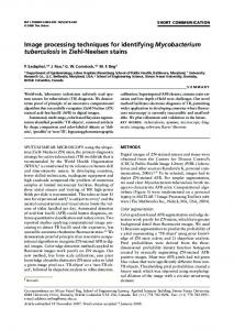
2. Preprocessing Some representative preprocessing examples are presented in Fig. 2 for a carbon fiber reinforced plastic (CFRP) specimen with 25 Teflon® insertions of different sizes (from 3 to 15 mm in lateral size, D) and at several depths (from 0.2 to 1.0 mm in depth, z). Fig. 2a shows the specimen geometry and Fig. 2b presents a raw thermogram (i.e. with no correction of any kind) at t=209 ms. The preprocessing techiques are discussed one by one in the following paragraphs, the corresponding results are shown in Fig. 2c to f. 2.1 Fixed Pattern Noise Fixed pattern noise (FPN) is the result of differences in responsivity of the detectors to incoming irradiance. It is a common problem when working with focal plane arrays (FPA). FPN for a particular configuration can be recovered from a blackbody image for later subtraction from the thermogram sequence. Fig. 2c shows an example of FPN extracted from a blackbody image at 18oC, using a Santa Barbara focal plane camera (model SBF125) operated at 157 Hz. The result of subtracting Fig. 2c (FPN) from Fig. 2b (raw thermogram) is shown in Fig. 2f. This image was also corrected for vignetting and badpixels as explained next. 2.2 Badpixels A badpixel can be defined as an anomalous pixel behaving differently from the rest of the array. For instance, a dead pixel remains unlit (black) while a hot pixel is permanently lit (white). In any case, badpixels do not provide any useful information and only contribute to deteriorate the image contrast. A map of badpixels is generally known from the FPA manufacturer or they can be detected manually or automatically, the value at badpixel locations is then replaced by the average value of neighboring pixels.

IV Conferencia Panamericana de END

Buenos Aires – Octubre 2007

2

2.3 Vignetting Vignetting is another source of noise on thermograms that causes a darkening of the image corners with respect to the image center due to limited exposure. Vignetting depends on both pixel location and temperature difference with respect to the ambient. A correction procedure has been proposed [3]. Fig. 2d shows the vignetting correcting coefficients image for the SBF125 Santa Barbara camera operated at 157 Hz. Lateral size, D =

30 cm

A-A

3 mm A

5 mm

z= 1.0 mm

7 mm 10 mm

0.6

15 mm 30 cm

0.2 0.4 5 cm 0.8 5 cm

A

10 plies thick

4000

6000

(a)

8000

10000

12000

14000

-400

-200

(b)

0

200

400

600

(c)

Frame Rate = 157.83Hz, Integration Time = 1.244 ms 60

Temperature

50 40 30

Data T = -29.0339 + 0.014862g -1.4194e-006g2 + 7.7618e-011g3 -1.6834e-015g4

20 10 0 0

0

0.2

0.4

0.6

0.8

1

0.5

1 Gray level

1.5

2 4

x 10

22

23

24

25

26

27

28

(d) (e) (f) Fig. 2. (a) CFRP specimen with 25 Teflon® inclusions of different sizes and at several locations; (b) raw thermogram at t=209 ms after heat pulse; (c) FPN; (d) thermogram showing badpixels and the vignetting correcting coefficients; (e) temperature calibration curve (f) thermogram in (b) corrected for FPN, badpixels and vignetting and calibrated in temperature. 2.5 Temperature Calibration A transformation function have to be used to convert the gray scale values g provided by the infrared camera into a linearly incrementing physical quantity, e.g. temperature. The procedure [3] consists to position the IR camera in front of a reference temperature source (such as a blackbody or a thick Copper plate) brought to various known temperatures. As the reference temperature source is varied, the IR images are recorded. Average of the central pixels in the field of view allows to get the calibration curve through a polynomial fit. Fig. 2e presents a typical result. Fig. 2f shows a thermogram at t=209 ms corrected for FPN, badpixels and vignetting and calibrated for temperature. This thermogram still shows some background noise (vertical lines throughout the image) that was produced during data acquisition. It is possible to get ride of this distortion by subtracting a cold image (a thermogram acquired prior to the heat pulse) as in Fig. 4a. Notice that other features, e.g. part of the flash lamp at the left, are eliminated from the scene.



3

2.6 Noise Smoothing One of the most useful preprocessing (and postprocessing) techniques is noise smoothing. For instance, neighbor processing can be performed by passing a mask or kernel through the image. More elaborated noise removal techniques are available; see for instance Fig. 3. Fig. 3a and b show the results before and after applying the sliding Gaussian method [1], p. 196, respectively. Phase delay images or phasegrams (see section 3.2) where used. Data was obtained from a steel plate (50x100x2 mm3) with three flat-bottom holes having the same depth (z=1 mm) and area (25 mm2) but different geometry: 1x25 mm2, 2.5x10 mm2 and 5x5 mm2.

(a) (b) Fig. 3. (a) Unfiltered; and (b) filtered with a Gaussian (σ=2): spatial profiles through the defects (top); phasegrams (middle); and segmentation results using Canny’s method [2] for edge detection (bottom). Although all defects are visible with good contrast in both phasegrams in Fig. 3 (middle), the interest of using a Gaussian filter is quite evident in the spatial profiles (top) but especially in the segmentation results after the application of the Canny edge detector [2] Fig. 3 (bottom). Once data has been preprocessed, it is possible now to perform a procesing technique to enhance defect contrast for detection purposes.

3. Processing 3.1 Thermal Contrast Techniques Thermal contrast-based techniques are probably the most common way of processing thermographic data. Various thermal contrast definitions exist [1], p. 198, must of them share the need of a sound area Sa, i.e. a non-defective region within the field of view. For instance, the absolute thermal contrast ∆T(t) is defined as [1]: ∆T (t ) = Td (t ) − TSa (t )

(1)

with T(t) being the temperature at time t, Td(t) the temperature of a pixel p (defective or not) or the average value of a group of pixels, and TSa(t) the temperature at time t for the Sa. No defect can be detected at a particular t if ∆T(t)=0.



4

Establishing this Sa is the main drawback of thermal contrast especially if automated analysis is needed or if nothing is known about the specimen. Even when defining a Sa is a straightforward, considerable variations on the results are observed when changing the location of Sa [4]. See for instance Fig. 4a, which shows the thermal contrast profiles (bottom) for the four different sound areas around a defect shown in the thermogram (top). As can be seen, there are significant variations in thermal contrast profiles even though the selected sound areas are not far from each other and from the defect. The spatial profile on top of Fig. 4a provides an indication of non-uniform heating, the right side of the specimen is at higher temperature (up to 3oC) than the left.

S a1 Sa3 defect

Sa4

0

1

2

3

4

Sa2

5

-0.2

6

-4

0

0.2

0.4

0.6

-1.2 S

S

a1

-3

-1

S

S

-0.8

S

a2

a2

S

-2

a4

-1

∆T [ oC]

a3

∆T [ oC]

a1

S

a3

S

a4

-0.6 -0.4 -0.2

0 0 1

.01

.1

1

6.3

0.2

.01

t [s]

.1

1

6.3

t [s]

(a) (b) Fig. 4. Spatial profiles (top), thermograms at t=209 ms (center), and thermal contrast profiles for 4 different Sa definitions (bottom), for: (a) thermogram in Fig. 2f after cold image subtraction; and (b) DAC result. The problem of Sa location was recently solved with the differential absolute contrast (DAC) [5], in which, instead of looking for a non-defective area, an ideal Sa temperature at time t is computed locally assuming that on the first few images (at least one image at time t’ in particular, see below) this local point behaves as a Sa. The first step is to define t’ as a given time value between the instant when the pulse has been launched, and the precise moment when the first defective spot appears in the thermogram sequence, i.e. when there is enough contrast for the defect to be detected. At t’, there is no indication of the existence of a defect yet. Therefore, the local temperature for a Sa is exactly the same as for a defective area [6]:

TSa (t ′) = Td (t ′ ) =

Q

(2)

e π ⋅ t′

By substituting Eq. (2) into the absolute contrast definition, Eq. (1), it follows that :



5

∆TDAC = Td (t ) −

t′ ⋅ T (t ′) t

(3)

Actual measurements diverge from the solution provided by Eq. (3) for later times and as the plate thickness increases with respect to the non-semi-infinite case. Nevertheless, the DAC technique has been proven to be very effective as it reduces the artefacts caused by non-uniform heating and surface geometry even for the case of anisotropic materials at early times [7], Fig. 4b shows a good exemple. As can be observed, nonuniform heating was drastically reduced when compare to Fig. 4a (see the spatial profiles and the thermograms), and the defect contrast is imporved as a result. The thermal contrast profiles for different locations show little variation at early times (up to 1 s), and then they diverge. A modified DAC technique has been proposed [8] to extend the validity of the DAC result to later times. It is based on a finite plate model and the thermal quadrupoles theory that includes the plate thickness L explicitly in the solution to extend the validity of the DAC algorithm to later times. The Laplace inverse transform is used to obtain a solution of the form [8]:

∆TDAC ,mod (t ) = Td (t ) −

 l −1 coth 

pL2   α  t

 l coth 

pL2   α  t'

−1

⋅ T (t ' )

(4)

where p is the Laplace variable. 3.5 Thermographic Signal Reconstruction

Thermographic signal reconstruction (TSR) [9] is an attractive technique that allows increasing the spatial and temporal resolution of a sequence, while reducing the amount of data to be manipulated. TSR is based on the assumption that temperature profiles for non-defective pixels should follow the decay curve given by the 1D solution of the Fourier equation - Eq. (2) - which may be rewritten in the logarithmic form as [9]:

Q 1 ln (∆T ) = ln   − ln (πt ) e 2

(5)

Eq. (2) however, is only an approximation of the solution for the Fourier equation. To fit the thermographic data, it has been proposed [9] to expand the logarithmic form into a series by using a m-degree polynomial of the form: ln (∆T ) = a0 + a1 ln (t ) + a 2 ln 2 (t ) + ... + a n ln n (t )

(6)

The thermal profiles corresponding to non-defective areas in the sample will approximately follow a linear decay, while a defective area will diverge from this linear behaviour. Typically, m is set to 4 or 5 to assure a good correspondence between acquired data and fitted values while reducing the noise content in the signal. At the end, the entire raw thermogram sequence is reduced to m+1 coefficient images (one per polynomial coefficient) from which synthetic thermograms can be reconstructed. Fig. 5 presents the five images corresponding to the coefficients of a 4th degree polynomial used for fitting preprocessed data (without cold image subtraction) as in Fig. 2f. It is



6

possible to detect 23 of the 25 inclusions. The last two coefficients show the background noise (vertical lines).

(a) (b) (c) (d) (e) Fig. 5. Coefficient images of a 4th degree polynomial used for fitting preprocessed data (without cold image subtraction) as in Fig. 2f. Synthetic data processing brings interesting advantages such as: significant noise reduction, possibility for analytical computations and data compression (from N to m+1 images). As well, analytical processing provides the possibility of estimating the actual temperature for a time between acquisitions from the polynomial coefficients. Furthermore, the calculation of first and second time derivatives from the synthetic coefficients is straightforward [9]. The first time-derivative indicates the rate of cooling while the second time-derivative refers to the rate of change in the rate of cooling. Therefore, time derivatives are more sensitive to temperature changes than raw thermal images. There are no purpose using derivatives of higher order; since, besides the lack of a physical interpretation, no further improvement in defect contrast is obtained. 3.2 Pulsed Phase Thermography In pulsed phase thermography (PPT) [10], data is transformed from the time domain to the frequency spectra using the one-dimensional discrete Fourier transform (DFT) [2]: N −1

Fn = ∆t ∑ T (k∆t )exp ( − j 2πnk k =0

N)

= Re n + Im n

(7)

where j is the imaginary number (j2=-1), n designates the frequency increment (n=0,1,…N), ∆t is the sampling interval, and Re and Im are the real and the imaginary parts of the transform, respectively. Real and imaginary parts of the complex transform are used to estimate the amplitude A, and the phase φ, [11]: An = Re n2 + Im2n

and

 Imn    Re n 

φn = tan −1 

(8)

DFT can be applied to any waveform, hence it can be used with pulsed, lock-in and vibrothermography data. The phase, Eq. (8), is of particular interest in NDE given that it is less affected than raw thermal data by environmental reflections, emissivity variations, non-uniform heating, and surface geometry and orientation. These phase characteristics are very attractive not only for qualitative inspections but also for quantitative characterization of materials as will be pointed out in section 4. Fig. 6 shows five phasegrams at different frequencies. Non-uniform heating (and surface shape) have little impact on phase. Deep features, visible at low frequencies, “disappear” at higher frequencies. For instance, the line of defects at z=1.0 mm



7

(topmost, refer to Fig. 2a), is visible in Fig. 6a but it is no longer visible in Fig. 6b. The line of defects at z=0.8 mm is no longer visible in Fig. 6c, and so on. Even though all defects in a line have different sizes, all defects are detected at about the same frequencies.

(a) (b) (c) (d) (e) Fig. 6. PPT results: phasegrams at f= (a) 0.15; (b) 0.47; (c) 0.63; (d) 1.10; and (e) 2.21 Hz. As any other thermographic technique, PPT is not without drawbacks. The noise content is considerable, especially at high frequencies. A de-noising step is therefore often required, as illustrated in Fig. 3. The combination of PPT and TSR is another possibility, reducing noise and allowing the depth retrieval of defects [12]. Another difficulty is that, given the time-frequency duality of the Fourier transform, a special care must be given to the selection of the sampling and truncation parameters prior to the application of the PPT. These two parameters depend on the thermal properties of the material and on the depth of the defect, which are often precisely the subject of the investigation in hand. An interactive procedure has been proposed for this matter [13]. 3.3 Principal Component Thermography The Fourier transform provides a valuable tool to convert the signal from the temperature-time space to a phase-frequency space but it does so through the use of sinusoidal basis functions, which may not be the best choice for representing transient signals (as the temperature profiles typically found in pulsed thermography). Singular value decomposition (SVD) is an alternative tool to extract spatial and temporal data from a matrix in a compact or simplified manner. Instead of relying on a basis function, SVD is an eigenvector-based transform that forms an orthonormal space. SVD is close to principal component analysis (PCA) with the difference that SVD simultaneously provides the PCAs in both row and column spaces. The SVD of an MxN matrix A (M>N) can be calculated as follows [14]: A=URVT

(9)

where U is a MxN orthogonal matrix, R being a diagonal NxN matrix (with singular values of A present in the diagonal), VT is the transpose of an NxN orthogonal matrix (characteristic time). Hence, in order to apply the SVD to thermographic data, the 3D thermogram matrix representing time and spatial variations has to be reorganised as a 2D MxN matrix A. This can be done by rearranging the thermograms for every time as columns in A, in such a way that time variations will occur column-wise while spatial variations will occur row-wise. Under this configuration, the columns of U represent a set of



8

orthogonal statistical modes known as empirical orthogonal functions (EOF) that describe the data spatial variations. On the other hand, the principal components (PCs), which represent time variations, are arranged row-wise in matrix VT. The first EOF will represent the most characteristic variability of the data; the second EOF will contain the second most important variability, and so on. Usually, original data can be adequately represented with only a few EOFs. Typically, a 1000 thermogram sequence can be replaced by 10 or less EOFs. Fig. 7 shows the first five EOFs for a cropped portion of the CFRP specimen obtained after applying PCT. Two cases were considered: uncorrected data (top), as in Fig. 2b; and preprocessed data with cold image subtraction (bottom), as in Fig. 4a. Later EOFs show only noise. For the uncorrected case, the first image (EOF1) shows the vignetting effect and the FPN. The FPN is still present at the second image (EOF2), but it no longer shows any vignetting, non-uniform heating shows up instead. Interestingly, the next three EOFs do not present any of these degradation sources, only defects and the specimen fiber matrix are seen. From these three images it is possible to detect 22 of the 25 Teflon® inclusions. For the case when PCT is applied to preprocessed data, there is no vignetting or FPN but is still strongly affected by non-uniform heating. Non-uniform heating is well distinguished in EOF1 but is no longer visible on later EOFs. Defect visibility is improved with respect to the uncorrected case; it is possible now to detect 24 of the 25 inclusions with EOF2 to EOF5, and the fiber matrix can be seen in EOF2.

(a) (b) (c) (d) (e) Fig. 7. PCT results for the case of uncorrected data (top) as in Fig. 2a, and for preprocessed data (bottom) with cold image subtraction as in Fig. 4a: (a) EOF1; (b) EOF2; (c) EOF3; (d) EOF4; and (e) EOF5. The techniques presented up to this point are intended to enhance the contrast of the thermographic data.. The next step is the characterization of the inspected specimen, i.e. to detect the defects, to determine its thermal properties, size and depth. Some inversion techniques have been proposed for this matter as discussed next.

4. Quantification 4.1 Defect Detection Algorithms Several approaches are possible in detection. Manual identification by an experienced observer is the most common. NDT organizations around the world have issued



9

personnel qualification and certification standards. For instance, the American Society of Nondestructive Testing (ASNT) recommends a three level training certification for infrared testing personnel [15], p. 15. On the automated side, different algorithms have been proposed. Thresholding (of processed - contrast, PPT, PCT, TSR - images) is common. Edge detector operators such as Sobel, Roberts, Canny, etc. [2] are also common as shown in Fig. 3, in which a Canny edge detector was used for segmentation. Signal filtering can help to improve results. 4.2. Depth Inversion Methods 4.2.1 Thermal Contrast Several methods have been proposed [1], chap. 10. All rely on a sort of calibration either with a thermal model or with various specimens representative of unknown ones. For instance, one can compute defect depth z by extracting a few parameters on the thermal contrast curve such as the maximum contrast ∆Tmax and its time of occurrence tmax [16]: 12 h z = A ⋅ t max ⋅ ∆Tmax

(10)

with parameters A and h obtained from the calibration process. Other empirical relationships have been proposed for thermal resistance R, which is proportional to defect thickness. 4.2.2 Statistical Models Statistical behavior of regions of interest such as background and defects has also being exploited for depth classification. The principle is that temperature, phase and amplitude can be modeled under some circumstances (such as in case of “white” noise sources) by a Gaussian random process [1], p. 417. First a calibration or “learning phase” in which data images with defects of known depths and background location are made available so that local means m and standard deviation σ are computed at each time increment and for each zone of interest (background and known defects). In the subsequent analysis step, unknown pixels are analyzed and individual probabilities are computed with m and s for a given pixel to be part of a given class. Assuming statistically independent events, individual probabilities (at different time increment) can be multiplied together to form a global probability. The winning rule is then simple: the largest wins. 4.2.3 Blind frequency It has been observed from experimental data that a linear relationship exists between defect depth z, and the inverse square root of the blind frequency fb1/2, i.e. the frequency at which the phase contrast is enough for a defect to be visible [17]. The thermal diffusion length expressed by [18]: µ=(2α/ ω), with α=k/ρcP being the thermal diffusivity and ω=2πf the angular frequency, can be used to fit experimental data [19]:

z = C1

α π fb

+ C2

(11)

where C1 is an empirical constant and fb [Hz] is the blind frequency.



10

It has been observed that, C1=1 when using amplitude data, whilst reported values when working with the phase are in the range 1.5