THETO — A Fast and High-Quality Partitioning Driven ... - CiteSeerX

T HETO — A Fast and High-Quality Partitioning Driven Global Placer ∗

Navaratnasothie Selvakkumaran and George Karypis Department of Computer Science and Engineering, Digital Technology Center and Army HPC Research Center, University of Minnesota, Minneapolis {selva,karypis}@cs.umn.edu

ABSTRACT

Keywords

Partitioning driven placement approaches are often preferred for fast and scalable solutions to large placement problems. However, due to the inaccuracy of representing wirelength objective by cut objective the quality of such placements often trails the quality of placements produced by pure wirelength driven placements. In this paper we present T HETO, a new partitioning driven global placement algorithm that retains the speed associated with traditional partitioning driven placement algorithms but incorporates a number of novel ideas that allows it to produce solutions whose quality is better than those produced by more sophisticated and computationally expensive algorithms. The keys to T HETO’s success are a new terminal propagation method that allows the partitioner to better capture the characteristics of the various cut nets and a new post-bisectioning refinement step that enhances the effectiveness of the new terminal propagation. Experiments on the ISPD98 benchmarks shows that T HETO produces global placement solutions that are 6% better in terms of the half perimeter wirelength than Dragon while requiring significantly less time.

Partitioning, Placement, wirelength objective

Categories and Subject Descriptors B.7.2 [Integrated Circuits]: Design Aids

General Terms Algorithms, Experimentation ∗ This work was supported in part by NSF CCR-9972519, EIA9986042, ACI-9982274, ACI-0133464, and ACI-0312828; the Digital Technology Center at the University of Minnesota; and by the Army High Performance Computing Research Center (AHPCRC) under the auspices of the Department of the Army, Army Research Laboratory (ARL) under Cooperative Agreement number DAAD19-01-2-0014. The content of which does not necessarily reflect the position or the policy of the government, and no official endorsement should be inferred. Access to research and computing facilities was provided by the Digital Technology Center and the Minnesota Supercomputing Institute.

1. INTRODUCTION Placement is one of the fundamental problems in physical design and numerous algorithms have been developed utilizing a variety of ideas and optimization techniques. However, the ever increasing problem sizes and shortening time-to-market windows require scalable and high-quality solutions in minimal amount of time. These pressures were largely limited to ASIC placement in the past, but modern FPGAs have grown to match the size of ASICs, which necessitates the development of extremely fast global placement algorithms, in order to facilitate reasonable compile times demanded by FPGA users. This has led to the re-emergence of partitioning driven placement (PDP) methods, as advances in circuit partitioning resulted in placement algorithms that are computationally scalable, capable of leading to high-quality solutions, and can scale to very large designs. Examples of such partition driven placement tools includes Capo [4], Dragon [14], and FengShui [1] that provide different time-quality trade-offs. In this paper we present T HETO, a new top-down hierarchical partitioning driven global placement algorithm that incorporates a number of novel ideas to further improve the quality of the placement solution. Our key contributions are the following: (i) a new method for terminal propagation that takes into account the size of the bounding boxes of the various nets; (ii) a new step in the overall structure of the hierarchical partitioning driven placement framework that further improves the quality of the bisections after the computation of each level; (iii) a comprehensive experimental evaluation of various algorithmic choices for partitioning driven placement and their impact on both quality and computational requirements. Using the placement benchmarks derived from the ISPD98 benchmark [8] we show that T HETO is able to produce solutions whose wirelength are on the average up to 6% better in terms of half-perimeter wirelength than the solutions produced by Dragon (one of the best performing schemes [1]). In addition, T HETO has very low computational requirements, making it one of the fastest high-quality partitioning driven placement algorithms. The rest of this paper is organized as follows. Section 2 provides some definitions and introduces the notation that is used throughout the paper. Section 3 describes T HETO and provides details about the various algorithms that it uses. Section 4 evaluates T HETO’s performance and compares it against other schemes. Finally, Section 5 provide some concluding remarks.

2. BACKGROUND .

The partitioning-driven global placement (PDP) paradigm is a

divide-and-conquer strategy used to combinatorially partition the netlist and assign the partitions to corresponding geometrically subdivided bins on the two dimensional chip surface. We say this process is applied at multiple levels of global placement, which simply means that we successively solve global placement for finer and finer bin sizes. At the top level, there is only one bin encompassing the entire area of the chip, and all the movable cells of the netlist are at the center of this bin. In the next level, there are two bins which contain bisected portions of the netlist. In the subsequent third level, each of these bins are further subdivided which results in 4 bins. This process continues until there are 2 m ∗2n bins, which is called bottom level. A netlist G = (V, E) is a set of cells V and a set of nets E. Each net is a subset of the set of cells V . The size of a net is the cardinality of this subset. A cell v is said to be incident on a net e, if v ∈ e. Each cell v and net e has a weight associated with them and they are denoted by w(v) and w(e), respectively. Pin is the location on the cell that physically attaches the net to the cell. The external portion of a net is a subnet induced by the cells incident on the net but lie outside the bin currently being considered. Similarly external cells of a net are the cells that are incident on the external portion of that net. Topological neighbors of a cell v are the subset of cells that are incident on at least one of the nets, on which v is also incident. The quality of the placement is measured in terms of the halfperimeter wirelength (HPWL), which is equal to the weighted sum of half-perimeters of the bounding boxes of the nets that enclose the cells incident on each net, i.e., HP (e) ∗ w(e). The wirelength objective of the global placement is to minimize HPWL, while satisfying upper- and lower-bound constraints on the total weight of cells that each of the bins contains (balance constraint).



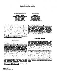
3. THE T HETO PLACER Our placement algorithm, called T HETO, follows the general top-down hierarchical partition driven placement framework. The overall structure of the computation performed at each level of the hierarchy is shown in Figure 1. They consist of three distinct steps. The first step computes a bisection of each bin using a cut-based hypergraph partitioning algorithm. The second step, which is applied after each bin has been bisected, further improves the cut (and to some extent the wirelength) of the original bisection by taking into account the finer-level partitioning of all the bins. Finally, the last step focuses on minimizing the wirelength of the placed solution at the current level of the hierarchy, by moving cells between the bins so that to reduce the half-perimeter wirelength. To a large extent T HETO’s structure is similar to that used by previously developed placement algorithms [14, 4, ?], with the only major difference being the introduction of the post-bisection refinement step. As we will later see in the experimental results section, this step significantly improves the quality of the placement and is instrumental in contributing to T HETO’s overall effectiveness. In the rest of this section we describe various schemes that we developed and evaluated for performing each one of these three steps.

3.1 Partitioning the bins T HETO bisects each bin using a multilevel hypergraph partitioning algorithm that was derived from hMetis [11]. Multilevel partitioning algorithms are the current state-of-the-art and have been shown to find high-quality partitionings in moderate amount of time. Our locally modified version of hMetis retains its basic overall structure but it has been extended to accept real numbers as net weights and small balance tolerances. In addition, to further reduce the amount of time spent in partitioning we do not perform any V -

Start

Partition Bins No

Post-Bisect Refinement

Bottom Level?

DP Yes

Level-wise Refinement

Figure 1: The structure of our PDP algorithm T HETO

cycles and we have reduced the number of coarsening levels that is being computed. In general, the quality of our locally modified version is comparable to that of hMetis 1.5.3, which is available publically.

3.1.1

Terminal Propagation

Besides the partitioning algorithm itself, another key factor that affects the overall performance of partitioning driven placement is the method that is used to take into account the external portion of the nets that are incident on cells of the bin that is being currently bisected. The goal of these methods is to utilize the information that is external to the bin in an effort to bias the min-cut objective toward minimizing HPWL. T HETO achieves this by employing a scheme that is based on the widely used technique of terminal propagation (TP) [5] that also takes into account the bounding boxes of the various nets that are connected to cells that are outside the current bin. Traditionally, terminal propagation is performed as follows [3]. For each net that connects internal and external cells and lies exclusively on one half region of the area to be bisected, a fixed dummy cell is added (terminal propagated) to the child bin on that side to try to prevent that net from being extended to the other side (i.e., prevent it from being cut). For computational efficiency [4], instead of assigning a fixed dummy cell to each such net, only two fixed dummy cells are maintained, one for each partition and all the nets that require terminal propagation are attached to these dummy cells. We will refer to this scheme as traditional terminal propagation. One major deficiency of this scheme is that the assignment of uniform partitioning cost to all the nets (same weight), while in reality the magnitude of HPWL degradation does vary for each net cut. To illustrate this, consider the example shown in Figure 2, which graphically depicts the current state of the bisectioning process of three large bins in a local region of the chip. The top bin has already been bisected into children bins A1 and A2 , the bottom bin C0 has not yet been bisected, while the bin in the middle B 0 is being currently bisected. Let us say the largest x coordinate of external cells of a net is equal to X1 (connected to some cell A1 ), then if this net is cut then it would extend the bounding box by X2 − X1 , but on the other hand if the largest coordinate is equal to X0 (connected to some cell in C0 ) then if this net is cut the bounding box will only expand by X 2 − X0 which is half as much as X2 − X1 . The traditional terminal propagation scheme does not capture this anomaly, which can easily be accounted for by proper

Bin A1

Bin A2

cells

cells Bin B0

B1

cells

B2

Bin C0

3.3 Algorithms for Level-wise Improvement

cells X1

X0

V-cycle refinement. We will refer to this as the Repartition-based approach. Finally, unlike the earlier schemes that minimize the min-cut of the bisections, the third scheme that we developed tries to directly optimize the HPWL of the solution [7] using an FMbased refinement algorithm. Since, the initial bisection produced by hMetis when coupled with BBTP is already a good quality bisection for HPWL, we did not implement this refinement algorithm in a multilevel framework. We will refer to this as the WLFM-based approach.

X2

Figure 2: A Snapshot of partitioning the bins

net-weighting. For this reason we developed a bounding box aware terminal propagation scheme, denoted by BBTP, that explicitly weights the nets according to the degradation in the HPWL that can potentially occur if they get cut. Due to the cut direction being parallel to one of the axis (in our example parallel to Y axis), this can be accomplished by a simple heuristic. We first estimate the maximum x coordinate xmax and the minimum x coordinate xmin of the external cells. If (X2 − xmax ) > (xmin − X1 ) then we attach the net to fixed dummy cell located at bin B1 (X1 ), and set the netweight as w(e) ∗ ((X2 − xmax )/(X2 − X1 )). Similar logic applies for attaching the nets to fixed dummy cell located on the other bin (B2 ). An interesting, but traditionally ignored case occurs when there are ties (xmin = xmax = X0 ), in which case if the net is not cut, irrespective of which child bin it is located, the bounding box is always going to be half as much as X2 − X1 , but if it is cut the expansion of the bounding box is going to be X 2 − X1 . So the difference between the net being cut and not cut is half as much as X2 − X1 . Therefore, for these nets we set the weight as 0.5 ∗ w(e). When compared to traditional TP, this scheme captures the HPWL objective more accurately and works well even in the presence of fixed cells/pads that may be located anywhere on the chip.

3.2 Post-Bisection Refinement During the course of bisecting the various bins at each level of the hierarchy, the final locations of the cells at that level are known only for those bins that already have been bisected. As a result, terminal propagation cannot achieve its full potential in accounting for the external portions of the nets. The post-bisection refinement step introduced in T HETO is designed to address this problem as it is being applied once all the bins have been bisected and attempts to further improve the quality of each individual bisection and further reducing the HPWL either implicitly or explicitly. T HETO implements three different schemes for performing this post-bisection refinement. The first scheme performs a V-cycle refinement [12] at each bisection using the multilevel FM-based refinement algorithm implemented in hMetis. Specifically, it visits the different bisections in a random order and apply a single Vcycle refinement step. We will refer to this as the V-cycle-based approach. A limitation of this V-cycle-based approach is that it is biased towards the initial bisection, which may make it difficult to find a better solution (i.e., climb out of a local minima). For this reason, the second scheme that we implemented computes an entirely new bisection for each bin [4] and is further refined using a

The final step that T HETO performs at each level of the hierarchy is to directly focus on the HPWL objective and minimize it by performing a k-way refinement. In the course of this refinement individual cells are allowed to move between the bins as long as such moves will eventually lead to lower HPWL. In T HETO we developed three level-wise algorithms. First algorithm is a randomized swap based algorithm (we call it RSwap), which is expected to succeed in tight balance constraints compared to a single move. The second algorithm is a randomized move based algorithm(we call it RMove). For these two algorithms we utilize topology of the netlist to identify nearby cell to swap with or nearby bin to move to and make the swap or move greedily. For swap, topological neighbors become candidates for swap, while for move, the bins of the topological neighbors become candidate destinations. The reason for implementing them based on topology is due to the inherent efficiency (time complexity is linear in terms of the number of pins). We traverse the netlist repeatedly until no more swap or move is possible. Usually these algorithms converge in a few iterations. Drawing motivation from [10], we developed the third algorithm, in which we apply WLFM to two randomly chosen geometrically adjacent bins (We call this PairWLFM). In alternative iterations we pick the pairs to form diagonal and non-diagonal bins. Although this is a relatively expensive algorithm, it requires only a few such iterations.

3.4 Bin Legalization In T HETO, we predominantly address bin legalization by explicitly setting tight balance constraints for the partitioner. Despite that, bins tend to overflow when the number of cells being bisected is small. This is due to the inherent limitation of FM algorithm used in our partitioner. To handle such cases, we modified RMove algorithm to move the cells away from overflowing bins. We randomly pick the cells from the overflowing bin and evaluate the moves to their adjacent bins identified by the topological structure. The moves that result in least degradation in wirelength are taken until the balance constraint is satisfied. Even though this algorithm is not guaranteed to remove all the overflow (when there are very few cells and the adjacent bins are also in violation), in most cases it works quite satisfactorily. This heuristic could easily be extended to search for topological neighbors of depth greater than one if needed (as a topologically “chained” move or as a means to find more locations for move destination). Alternatively existing sophisticated legalization algorithms [15] can be used, which are really necessary only in the detail placement phase. T HETO’s bin legalization algorithm is always applied, when there were violations unless specified otherwise.

4. EXPERIMENTAL EVALUATION We evaluated the performance of the various algorithmic choices in T HETO on the placement benchmarks derived from the 18 ISPD98 circuits [8]. The number of cells and the number of nets in these

name ibm01 ibm02 ibm03 ibm04 ibm05 ibm06 ibm07 ibm08 ibm09

num cells 12282 19321 22207 26633 29347 32185 45135 50977 51746

num nets 11507 18429 21621 26163 28446 33354 44394 47944 50393

name ibm10 ibm11 ibm12 ibm13 ibm14 ibm15 ibm16 ibm17 ibm18

num cells 67692 68525 69663 81508 146009 158244 182137 183102 210323

num nets 64227 67016 67739 83806 143202 161196 181188 180684 200565

Table 1: The benchmark suite (IBMPlace v1.0).

benchmarks are shown in Table 1. Specifically, we used T HETO to compute the global placements for the first ten circuits (ibm01– ibm10) for 64 × 64 bins, and for the remaining circuits (ibm11– ibm18) for 128 × 128 bins. Note that these numbers are chosen to match the number of rows provided in each of these benchmarks. We have performed all our experiments on 1.5GHz Athlon MP processor machine. We have used gcc3.2 version with aggressive optimization (-O3 -ffast-math -funroll-all-loops -fomit-frame-pointer). The performance of the various schemes was evaluated by comparing two quantities. The first is the weighted half-perimeter wirelength (denoted as “HPWL” in the tables), which measures the quality of the solution in million units. T HETO uses weighted halfperimeter wirelength, so that net weighting based timing driven approaches can be seamlessly integrated. Solutions that have smaller HPWL values are better. The second is the amount of time required to compute the GP solution (denoted as “Time” in the tables). Schemes that require less time are preferred over those requiring more time. The numbers presented are average results of 10 independent runs. Also, to make overall comparisons between different schemes across the different data sets easier, we computed two summary statistics. The first is the total amount of time (denoted as “TTime” in the tables), which is simply the time required to place all 18 benchmarks. The second is called average quality relative to the best (denoted “AQB” in the tables) and measures the relative performance of the various schemes being compared in terms of HPWL. The AQB statistic for a particular scheme is computed as follows. For each benchmark we compute the ratio of the HPWL produced by that scheme against the smallest HPWL produced for that benchmark by any of the schemes under consideration, and we obtain its AQB by simply averaging these ratios across the 18 benchmarks. A scheme that achieved an AQB value that is 1.0 means that for all benchmarks it produced the smallest HPWL. In general, a scheme will outperform another, if its AQB value is smaller.

4.1 Evaluation of Various Algorithmic Choices As discussed in Section 3, there are a number of different algorithmic choices for each one of the three main steps within T HETO’s top-down hierarchical placement framework. In this section we present an experimental evaluation of these options and evaluate their impact on the overall GP solution. Due to space constraints, we are not able to provide an exhaustive comparison of all possible combinations for these steps. Instead, we provide comparisons of different alternatives for each step after making a reasonable choice for the other two phases.

4.1.1

Terminal Propagation Schemes

The performance achieved by the different terminal propagation schemes described in Section 3.1.1 is shown in Table 2. Specifically, this table shows the performance achieved by four differ-

ibm01 ibm02 ibm03 ibm04 ibm05 ibm06 ibm07 ibm08 ibm09 ibm10 ibm11 ibm12 ibm13 ibm14 ibm15 ibm16 ibm17 ibm18 AQB TTime

Traditional TP NRuns= 1 NRuns=5 HPWL Time HPWL Time 5.8 2 5.4 8 16.5 4 15.7 15 14.8 4 14.2 16 19.1 5 18.3 21 42.4 6 40.9 27 22.4 7 21.4 29 35.2 10 33.4 45 41.1 12 39.0 50 32.4 11 30.4 48 70.1 18 64.8 80 49.5 24 47.3 84 87.1 28 83.8 104 61.0 34 57.9 116 138.6 66 132.8 254 153.7 78 144.4 298 206.3 91 194.0 360 307.5 102 287.9 418 231.9 104 213.9 421 1.101 1.043 605 2395

BBTP NRuns=1 HPWL Time 5.4 2 15.6 4 14.1 4 18.4 5 40.6 7 21.8 7 33.1 11 37.0 13 30.3 12 64.2 19 47.2 25 82.8 30 58.7 36 134.3 71 149.4 84 199.7 99 298.9 112 214.2 114 1.045 657

NRuns=5 HPWL Time 5.2 8 15.0 17 13.6 18 17.6 23 39.5 33 20.7 32 31.9 49 35.7 57 29.0 52 62.5 86 45.3 89 79.7 111 56.0 123 128.4 276 143.1 319 189.3 378 283.0 453 198.5 454 1.000 2579

Table 2: Results obtained by terminal propagation schemes.

ent schemes. The first two schemes use the traditional terminal propagation scheme (labeled “Traditional TP”), whereas the other two are based on the new bounding box aware scheme (labeled “BBTP”). The difference between each pair of schemes is the number of different bisections that they compute during each bin-bisection step. In particular, the schemes labeled “NRuns=1” compute a single bisection, whereas the schemes labeled “NRuns=5” compute five different bisections and select the one that achieves the smallest cut. Note that all these experiments were performed without performing any bisection or level-wise refinement. From these results we can see that the new terminal propagation scheme is superior to the traditional approach as it leads to higher quality solutions without materially increasing the overall GP time. For example, when NRuns=1, BBTP leads to solutions that have 5.6% lower HPWL while incurring only a 10% degradation in time. Similar performance advantages can be seen for NRuns=5. Comparing the impact of improved bisectioning quality, we can see that it directly translates to lower HPWL. For example, when NRuns=5, the traditional TP results improved by 5.8% and the BBTP results improved by 4.5% while the runtime increased by a factor of four. Also, it is interesting to note that T HETO’s overall PDP engine is quite fast, as it can place the ibm01 benchmark (12K nets) in two seconds and the ibm18 benchmark (210K nets) within two minutes. Due to the quality advantage of BBTP with NRuns=5 and its modest computational requirements, we will use it as the default bin-bisectioning scheme in all our subsequent experiments.

4.1.2

Bisection Improving Schemes

The performance achieved by the different bin-bisection improvement schemes is shown in Table 3. Specifically, this table shows the performance achieved by three schemes described in Section 3.1, as well as the scheme that does not perform any bin-bisection refinement (labeled “BBTP5” as it corresponds to BBTP with NRuns=5). Note that all these experiments were performed without performing any level-wise refinement. From these results we can see that in terms of HPWL, the Repartition scheme performs the best among the bisection improving schemes, whereas the the V-Cycle and WLFM schemes produce solutions whose HPWL is about 3% and 2% worse than Repartition, respectively. In terms of computational requirements, the V-Cycle

ibm01 ibm02 ibm03 ibm04 ibm05 ibm06 ibm07 ibm08 ibm09 ibm10 ibm11 ibm12 ibm13 ibm14 ibm15 ibm16 ibm17 ibm18 AQB TTime

V-Cycle HPWL Time 5.1 11 14.9 22 13.4 24 17.7 31 38.3 44 20.3 44 31.0 69 35.0 84 28.4 79 60.3 123 44.0 130 77.9 161 54.7 183 126.7 398 137.9 477 183.5 555 272.1 629 194.6 653 1.021 3718

Repartition HPWL Time 5.0 19 14.5 37 13.2 39 17.1 51 37.8 72 19.7 69 30.5 109 34.3 126 27.9 117 59.4 195 43.0 201 76.2 254 53.6 280 122.7 620 136.6 727 180.8 896 268.4 1042 190.0 1029 1.000 5883

WLFM HPWL Time 5.1 17 15.1 80 13.5 42 17.6 54 39.1 107 20.2 79 30.6 111 34.6 203 28.3 129 63.6 237 44.0 249 79.8 361 54.5 346 128.0 784 140.2 984 184.6 1213 287.8 1548 194.3 1569 1.030 8112

BBTP5 HPWL Time 5.2 8 15.0 17 13.6 18 17.6 23 39.5 33 20.7 32 31.9 49 35.7 57 29.0 52 62.5 86 45.3 89 79.7 111 56.0 123 128.4 276 143.1 319 189.3 378 283.0 453 198.5 454 1.044 2579

Table 3: Results obtained by bisection improving schemes.

ibm01 ibm02 ibm03 ibm04 ibm05 ibm06 ibm07 ibm08 ibm09 ibm10 ibm11 ibm12 ibm13 ibm14 ibm15 ibm16 ibm17 ibm18 AQB TTime

RSwap HPWL Time 5.1 23 14.8 171 13.8 56 17.8 64 39.3 228 20.6 106 31.9 130 35.7 391 29.0 144 61.7 294 44.9 193 79.5 446 55.8 344 127.3 657 141.1 974 187.5 1310 278.7 1957 196.4 1852 1.027 9338

RMove HPWL Time 5.1 13 14.8 50 13.7 30 18.0 37 39.2 81 20.3 52 31.6 75 35.8 149 29.0 82 61.8 143 44.4 122 80.0 194 55.4 182 126.6 386 140.0 493 184.9 606 274.5 781 195.3 839 1.022 4316

PairWLFM HPWL Time 5.1 38 14.3 150 13.4 96 17.3 114 38.1 190 19.8 167 30.8 238 34.5 376 28.2 272 59.6 445 43.9 368 77.6 547 54.4 542 123.9 1107 139.2 1448 182.2 1733 271.0 2139 194.5 2195 1.000 12164

BBTP5 HPWL Time 5.2 8 15.0 17 13.6 18 17.6 23 39.5 33 20.7 32 31.9 49 35.7 57 29.0 52 62.5 86 45.3 89 79.7 111 56.0 123 128.4 276 143.1 319 189.3 378 283.0 453 198.5 454 1.033 2579

Table 4: Results obtained by level-wise refinement schemes.

scheme is the fastest, the WLFM scheme is the slowest, whereas the Repartition scheme is somewhere in between these two. Also, it is interesting to note that all three schemes lead to solutions whose HPWL is better than those achieved by BBTP5 alone. For example, the solutions produced by BBTP5 are about 4.4% worse than those produced by Repartition. These results indicate that there is a non-trivial quality advantage in introducing this new phase in the overall flow of PDP.

4.1.3

Level-Wise Refinement Schemes

The performance achieved by the different level-wise refinement schemes is shown in Table 4. This table shows the performance achieved by three schemes described in Section 3.3, as well as BBTP5, which does not perform any level-wise refinement. Note that all these experiments were performed without applying any bisection refinement. From these results we can see that the PairWLFM scheme achieves the best HPWL improvement compared to RSwap and RMove. The HPWL obtained by RSwap and RMove is about 3% and 2% higher

than that achieved by PairWLFM, respectively. However, PairWLFM’s performance advantage comes at a significant increase in the overall computational time. For example, PairWLFM requires five times more time than that required by BBTP5. Comparing the time required by different level-wise refinements, we can see that RMove is the fastest, requiring less than twice the time required by BBTP5. Finally, comparing the gains in HPWL achieved by this PDP step over the gains achieved by the bisection refinement step (Table 3) we can see that the later leads to higher improvements at a lower computational cost.

4.2 Overall Comparisons Our comparisons so far were focused on evaluating the various algorithmic choices for the three main steps of T HETO’s top-down hierarchical PDP flow. In this section we evaluate how the combination of some of these algorithmic choices affect the overall performance of T HETO. Table 5 shows the GP performance achieved by seven different schemes. The columns labeled “BBTP5”, “Repartition”, and “PairWLFM” correspond to the lowest HPWL achieving schemes identified in Sections 4.1.1–4.1.3. The column labeled “Repartition+PairWLFM” corresponds to the scheme that performs both bisection and level-wise refinements using the Repartition and PairWLFM schemes, respectively. The column labeled “V-Cycle + Repartition+WLFM” corresponds to the scheme that uses all three bisection refinement schemes one-after-the-other but does not perform an level-wise refinement. Finally, the scheme labeled “ALL” corresponds to the scheme that performs both bisection and levelwise refinement using all three bisection refinement schemes and all three level-wise refinement schemes applied one-after-the-other. In addition, the last column labeled “Dragon”, contains the GP results produced by Dragon [14]. We chosen Dragon for two reasons. First, it provides statistics regarding the quality of the GP solution that it computes, and second, based on a recent comprehensive comparisons of various placement algorithms [1, 16], Dragon produces either the highest quality or among the highest quality placement solutions. From these results we can see that as expected, the scheme that applies all the different algorithms bisection refinement and levelwise refinement (ALL) achieves the lowest HPWL and requires the most amount of time among the different possibilities for T HETO. However, the scheme that combines all bisection refinement schemes but performs no level-wise refinement (fifth column) achieves comparable HPWL results but is about 2.5 times faster. This observation is consistent with our earlier results in Section 4.1.3 that showed that the benefits achieved by level-wise refinement are usually smaller than those achieved by the bisection refinement algorithms. Comparing the results produced by T HETO against those produced by Dragon, we can see that all but the BBTP5 scheme produce GP solutions whose HPWL is slightly higher than those produced by Dragon. These gains range from about 2% up to 6%. Unfortunately, the times reported by Dragon cannot be directly compared as they correspond to Dragon’s overall GP run time, which also includes a “single cell switching” based hybrid phase as well as few more bisection levels for some of the benchmarks to aid DP. However, according the authors, the global placement phase is dominating its overall runtime [14]. As a result, we can infer that Dragon is much slower (in the range of 4–15 times slower) than the various instances of T HETO.

5. CONCLUSION In this paper we presented a new global placer algorithm that is based on the partitioning driven placement paradigm. We in-

ibm01 ibm02 ibm03 ibm04 ibm05 ibm06 ibm07 ibm08 ibm09 ibm10 ibm11 ibm12 ibm13 ibm14 ibm15 ibm16 ibm17 ibm18 AQB TTime

BBTP5 HPWL Time 5.2 8 15.0 17 13.6 18 17.6 23 39.5 33 20.7 32 31.9 49 35.7 57 29.0 52 62.5 86 45.3 89 79.7 111 56.0 123 128.4 276 143.1 319 189.3 378 283.0 453 198.5 454 1.080 2579

Repartition HPWL Time 5.0 19 14.5 37 13.2 39 17.1 51 37.8 72 19.7 69 30.5 109 34.3 126 27.9 117 59.4 195 43.0 201 76.2 254 53.6 280 122.7 620 136.6 727 180.8 896 268.4 1042 190.0 1029 1.034 5883

PairWLFM HPWL Time 5.1 38 14.3 150 13.4 96 17.3 114 38.1 190 19.8 167 30.8 238 34.5 376 28.2 272 59.6 445 43.9 368 77.6 547 54.4 542 123.9 1107 139.2 1448 182.2 1733 271.0 2139 194.5 2195 1.045 12164

Repartition+PairWLFM HPWL Time 4.9 47 14.1 161 13.2 109 16.7 136 37.4 214 19.5 193 30.0 278 33.5 428 27.5 325 58.5 537 42.7 458 76.0 640 53.3 655 119.6 1369 134.9 1739 176.7 2102 264.7 2593 185.8 2685 1.019 14670

V-Cycle+Repartition+WLFM HPWL Time 4.9 29 14.0 80 13.0 64 16.5 89 36.8 136 19.2 126 29.8 187 33.2 269 27.5 220 58.2 358 42.5 371 74.4 487 52.5 523 119.3 1304 132.9 1581 173.8 1904 260.6 2212 185.0 2288 1.008 12227

ALL HPWL Time 4.9 74 13.8 394 12.7 178 16.7 216 36.8 501 19.3 349 29.6 444 32.7 915 27.3 538 57.9 965 42.0 732 75.1 1274 52.2 1143 118.1 2413 132.1 3249 173.0 3987 257.2 5235 182.9 5475 1.002 28083

Dragon HPWL Time∗ 5.0 1243 15.0 1857 13.7 1509 17.7 1732 42.2 4413 20.8 3017 33.0 3479 36.0 4990 29.8 3859 60.5 8765 42.8 5678 73.5 9113 55.8 7301 123.8 14007 140.6 21135 180.1 22870 271.4 29785 197.6 26546 1.068 171301

Table 5: Results obtained by combining T HETO’s different parameters and from Dragon. troduced a number of different algorithmic choices for its various steps and presented a detailed experimental evaluation. Our results showed that min-cut partitioning alone when combined with effective terminal propagation can lead to global placement algorithms that are both fast and of high quality. In fact, our algorithm is able to produce global placement solutions whose half perimeter wirelength is up to 6% better when compared by other state-of-the-art academic placement tools.

6. REFERENCES [1] A.Agnihotri, M.C.Yildiz, A.Khatkhate, A.Mathur, S.Ono, and P.H.Madden. Fractional cut : Improved recursive bisection placement. In Proc. of ICCAD, pages 307–310, 2003. [2] A.B.Kahng and X.Xu. Local unidirectional bias for smooth cutsize-delay tradeoff in performance driven partitioning. In Proc. of ISPD, pages 81–86, 2003. [3] A.E.Caldwell, A.B.Kahng, and I.L.Markov. Optimal partitioners and end-case placers for top-down placement. In Proceedings of ISPD, pages 90–96, 1999. [4] A. A.E.Caldwell and I.L.Markov. Can recursive bisection alone produce routable placements? In Proc. of DAC, pages 477–482, 2000. [5] A.E.Dunlop and B.W.Kernighan. A procedure for placement of standard-cell vlsi circuits. In IEEE Trans. on CAD of Integrated Circuits and Systems, pages CAD–4(1):92–98, 1985. [6] C.Ababei, S.Navaratnasothie, K.Bazargan, and G.Karypis. Multi-objective circuit partitioning for cutsize and path-based delay minimization. In Proc. ICCAD, pages 181–185, 2002. [7] D.J-H.Huang and A.B.Kahng. Partitioning-based standard-cell global placement with an exact objective. In Proc. ISPD, pages 18–25, 1997. [8] http://er.cs.ucla.edu/benchmarks/ibm place/index.html. [9] J.Cong, M.Romesis, and M.Xie. Optimality, scalability and stability study of partitioning and placement algorithms. In Proc. of ISPD, pages 88–94, 2003. [10] J.Cong and S.K.Lim. Multiway partitioning with pairwise movement. In Proc. ICCAD, pages 512–516, 1998.

[11] G. Karypis, R. Aggarwal, V. Kumar, and S. Shekhar. Multilevel hypergraph partitioning: Application in vlsi domain. IEEE Transactions on VLSI Systems, 20(1), 1999. A short version appears in the proceedings of DAC 1997. [12] G. Karypis and V. Kumar. hMetis 1.5: A hypergraph partitioning package. Technical report, Department of Computer Science, University of Minnesota, 1998. Available on the WWW at URL http://www.cs.umn.edu/˜metis. [13] G. Karypis and V. Kumar. Multilevel algorithms for multi-constraint graph partitioning. In Proceedings of Supercomputing, 1998. Also available on WWW at URL http://www.cs.umn.edu/˜karypis. [14] X. M.Wang and M.Sarrafzadeh. Dragon2000: Standard-cell placement tool for large industry circuits. In Proc. of ICCAD, pages 160–163, 2000. [15] S.W.Hur and J.Lillis. Mongrel: Hybrid techniques for standard-cell placement. In Proceedings of ICCAD, pages 165–170, 2000. [16] T.F.Chan, J.Cong, T.Kong, J.R.Shinnerl, and K.Sze. An enhanced multilevel algorithm for circuit placement. In Proc. of ICCAD, pages 299–306, 2003.