hyperspecral data, we need a decision rule to fuse the individual ..... Sens., vol. 43, no. 3, pp. 441â454, Mar. 2005. [12] X. Jia and J. A. Richards, âSegmented .... 2012) and the IEEE GEOSCIENCE AND REMOTE SENSING MAGAZINE (2013).
668
IEEE JOURNAL OF SELECTED TOPICS IN APPLIED EARTH OBSERVATIONS AND REMOTE SENSING, VOL. 9, NO. 2, FEBRUARY 2016
Spectrometer-Driven Spectral Partitioning for Hyperspectral Image Classification Yi Liu, Student Member, IEEE, Jun Li, Member, IEEE, and Antonio Plaza, Fellow, IEEE Abstract—Classification is an important and widely used technique for remotely sensed hyperspectral data interpretation. Although most techniques developed for hyperspectral image classification assume that the spectral signatures provided by an imaging spectrometer can be interpreted as a unique and continuous signal, in practice, this signal may be obtained after the combination of several individual responses obtained from different spectrometers. In this work, we propose a new spectral partitioning strategy prior to classification which takes into account the physical design of the imaging spectrometer system for partitioning the spectral bands collected by each spectrometer, and resampling them into different groups or partitions. The final classification result is obtained as a combination of the results obtained from each individual partition by means of a multiple classifier system (MCS). The proposed strategy not only incorporates the design of the imaging spectrometer into the classification process but also circumvents problems such as the curse of dimensionality given by the unbalance between the high number of spectral bands and the generally limited number of training samples available for classification purposes. This concept is illustrated in this work using two different imaging spectrometers: the airborne visible infra-red imaging spectrometer, operated by NASA, and the digital airborne imaging system (DAIS), operated by the German Aerospace Center. Our experiments indicate that the proposed spectral partitioning strategy can lead to classification improvements on the order of 5% overall accuracy when using state-of-the-art spatial–spectral classifiers with very limited training samples. Index Terms—Airborne visible infra-red imaging spectrometer (AVIRIS), band reassignment, clustering, digital airborne imaging spectrometer, multiple classifier system (MCS), partitioning, spectrometer-driven classification.
I
I. I NTRODUCTION
MAGING spectroscopy (also called hyperspectral remote sensing) has experienced significant developments in recent years [1]. Currently, many sensors onboard airborne and spaceborne platforms are available, and these instruments keep collecting data from different locations on the surface of the Earth [2]. Hyperspectral data have been useful in many applications, including disaster monitoring, natural resources exploitation,
Manuscript received December 18, 2014; revised April 10, 2015; accepted May 11, 2015. Date of publication June 25, 2015; date of current version February 09, 2016. This work is supported by the National High Technology Research and Development Program of China (863 Program, No. 2013AA122303). (Corresponding author: Jun Li.) Y. Liu and A. Plaza are with the Hyperspectral Computing Laboratory, Department of Technology of Computers and Communications, Escuela Politécnica, University of Extremadura, Cáceres E-10071, Spain. J. Li is with Guangdong Provincial Key Laboratory of Urbanization and Geosimulation, Center of Integrated Geographic Information Analysis, School of Geography and Planning, Sun Yat-sen University, Guangzhou 510275, China. Color versions of one or more of the figures in this paper are available online at http://ieeexplore.ieee.org. Digital Object Identifier 10.1109/JSTARS.2015.2437614
and environmental applications. [3]–[5]. With the increasing spatial, spectral, and temporal resolutions of imaging spectrometers, the extremely high dimensionality and size of the data have become important concerns for hyperspectral data interpretation [6]. Among several techniques for hyperspectral image analysis, classification has been a very important research topic for interpreting hyperspectral data [7], in which the main challenges have been given by the unbalance between the high dimensionality of the data and the limited number of training samples generally available a priori [8]. In the following, we provide a description of the stateof-the-art in classification and spectral partitioning using the abbreviations introduced in Table I. Although supervised classification techniques such as the SVM [9] or MLR [10] have been shown to be quite successful for the interpretation of hyperspectral data (even in the presence of limited training samples), some techniques have taken advantage of dimensionality reduction [11]–[13] or subspace projection [14] prior to classification. The high existing correlation between bands has been exploited to design new methods for reducing data dimensionality, including methods that have found great popularity such as PCA [15], LDA [16], or MNF [17]. Subspace projection techniques such as HySime [18] have also been used for this purpose. In fact, it has been reported in previous works that classification after dimensionality reduction, subspace projection, or band/feature selection generally outperforms classification based on the full original hyperspectral data [19]. By reducing the number of bands, unsupervised feature selection [20], [21], semi-supervised feature selection [22], and supervised feature selection [23] have been reported to be able to achieve similar or better classification accuracies than using all available bands. Spectral partitioning, which is a form of dimensionality reduction, provides an alternative approach to deal with the high dimensionality of hyperspectral data. In comparison with traditional band reduction/selection approaches, a distinguishing feature of spectral partitioning is that all spectral bands of the input image can be used for the subsequent analysis process by creating multiple views of the original hyperspectral image. This can be achieved by selecting, for a given partition, a subset of bands that effectively subsamples the original spectral signature in the original hyperspectral scene while retaining its main characteristics. The selection of multiple disjoint subsamples provides multiple views of the original hyperspectral signature that can be combined for classification purposes. As reported in [24], this strategy can be implemented by using techniques such as AAP [25]), which first automatically generates spectral band clusters in which the spectral bands are correlated with
1939-1404 © 2015 IEEE. Personal use is permitted, but republication/redistribution requires IEEE permission. See http://www.ieee.org/publications_standards/publications/rights/index.html for more information.
LIU et al.: SD-SP FOR HYPERSPECTRAL IMAGE CLASSIFICATION
669
TABLE I L IST OF A BBREVIATIONS U SED IN T HIS PAPER
Fig. 1. Four spectrometers in the AVIRIS system (reproduced from [28]).
each other, and then the bands are reassigned from the clusters into new groups (namely spectral partitions), which constitute a subsampling of the original spectral signatures. Similarly, utilizing a bisection spectral partitioning strategy, the work in [26] reported a significant gain in classification performance for hyperspectral data. In [12], a spectral partitioning based on band correlation segmentation was also employed to achieve better results from the PCA transformation by performing the PCA on each partition (spectral segment). Besides, in [27], spectral and spatial partitioning were incorporated into PCA-based compressive projection for hyperspectral image reconstruction. These works indicate that spectral partitioning can lead to improved classification results for hypersepctral data. An important characteristic of spectral partitioning techniques such as those mentioned above is that they do not consider the physical characteristics of the imaging spectrometer, which may be critical in the process of creating the spectral band clusters. In fact, most classification techniques assume that the spectral signatures provided by an imaging spectrometer system for a given pixel can be considered as a unique and continuous signal. However, it is well known in hyperspectral imaging that different parts of the signal are subject to the different characteristics of the physical instruments after the combined individual responses from several different spectrometers. For instance, the AVIRIS1 system [28] is formed by four different spectrometers, covering the nominal spectral ranges: 400–700, 700–1300, 1300–1900, and 1900–2500 nm, respectively. As shown in Fig. 1, these four spectrometers (called A, B, C, and D, respectively) have completely different characteristics. For example, in the D spectrometer, a carefully specified linear variable blocking filter is used to limit the wavelengths 1 [Online]. Available: http://www.nasa.gov/centers/dryden/research/AirSci/ER2/aviris.html
of light for each element in the detector array. This specialized filter is intended to separate different spectral orders. For the A spectrometer, a 32-element silicon detector array with a blue enhanced response is used. The B, C, and D spectrometers each has 64-element arrays instead. As a result, our main contribution in this work is a new partitioning framework that is driven by the characteristics of the imaging spectrometer and its physical configuration, instead of assuming that the spectral signature is a continuous signal. The methodology that we propose in this work offers a new perspective that gives a new flavour to the problem of spectral partitioning. Given the fact that different spectrometers have different characteristics, our speculation in this work is that the conventional assumption that the spectral signatures can be interpreted as unique and distinct signals may not hold in all cases (at least, given the current status of hyperspectral technology), and that the use of a spectrometer-driven partitioning strategy prior to classification may lead to improved hyperspectral data interpretation results, in particular, when spectral partitioning is used for dimensionality reduction purposes. Similar observations can be made for other widely used imaging spectrometers, such as DAIS 79152 [29], ARES [30], Hyperion [31], or HyMap [32], among several others [2]. In this work, we develop a new spectrometer-driven partitioning strategy that considers the differences between the individual spectrometers in the spectral partitioning step. An important consideration of our approach is that, as the dimensionality of each spectrometer signal is much smaller than the whole spectral signal, it allows for the design of a subsequent classification system that is efficient in scenarios in which limited training samples are available a priori, as the system uses multiple views of the original spectral signatures but with reduced dimensionality, which allows for the classification of the original 2 [Online].
Available: http://www.uv.es/leo/daisex/Sensors/DAIS.htm.
670
IEEE JOURNAL OF SELECTED TOPICS IN APPLIED EARTH OBSERVATIONS AND REMOTE SENSING, VOL. 9, NO. 2, FEBRUARY 2016
hyperspectral data without discarding any information collected by the imaging spectrometer. In other words, instead of extracting features or removing bands, we reduce the dimensionality by reassigning the original bands into multiple views of the original data (according to the properties of the considered imaging spectrometer) and then using an MCS that considers all the information in the final classification. For comparative purposes, the proposed spectrometer-driven partitioning strategy is compared with random partitioning and with another previously developed method (the AAP), which relies on statistical principles rather than physical principles related to the imaging spectrometer. The concept is illustrated using two different systems: AVIRIS and DAIS 7915. This paper is organized as follows. In Section II, we introduce our spectral partitioning and classification framework, which is implemented using both the AAP clustering technique and our newly developed SD-SP strategy. This section also provides a comparison of these two spectral partitioning strategies to the simple random selection case to illustrate the differences obtained between using a statistical-driven method (the AAP) and a more physically driven method. Section III provides experimental results using representative data sets collected by the AVIRIS and DAIS 7915 systems. Finally, Section IV concludes with some remarks and hints at plausible future research lines. II. P ROPOSED F RAMEWORK In this section, we describe the proposed framework for hyperspectral image classification after spectral partitioning. Our framework is illustrated in Fig. 2. First, the original hyperspectral image is partitioned using spectral band clustering. For this purpose, we use two different strategies: AAP [25] (driven by statistical principles) and a newly proposed spectrometerdriven approach (which is more driven by physical principles related to the design of the imaging spectrometer). The resulting q partitions provide multiple views of the original spectral signatures in the hyperspectral data. These different views are classified using an MCS which is based on a probabilistic classifier: the subspace MLR (MLRsub) classifier in [14]. In the following, we first describe the two spectral band clustering techniques considered (providing a comparison between them) and then provide details about the considered MCS system. A. Spectral Band Clustering Using AAP-SP The AP method [33] was originally presented to automatically search for the optimal number of clusters in the analyzed data. A main contribution of the algorithm with regard to traditional unsupervised clustering approaches such as k-means [34] or ISODATA [35] is that the AP is less sensitive to initialization as it takes every sample as a potential cluster center. An adaptive version of AP (AAP) was proposed to automatically search for the optimal cluster number while removing inconsistencies [25]. As opposed to k-means or Isodata clustering, in AAP, all data points are simultaneously considered as potential exemplars, but exchange deterministic messages until a good set of exemplars gradually emerges. In other words,
Fig. 2. Proposed framework for spectral partitioning and classification of hyperspectral data.
using AAP we can perform band clustering without knowing in advance the number of exemplars. Let c be the number of band clusters and let ρ be the number of spectral partitions. In our previous work [24], we have adopted the AAP with a nested recursive iteration process for hyperspectral band clustering. Resulting from this process, the original hyperspectral data are divided into c-band clusters/groups, each of which contains a group of spectral bands with high similarity/correlation. After obtaining the c-band clusters, we then reassign the bands with high similarity/correlation to spectral partitions by a band reassignment algorithm described in Section II-B such that each partition contains the same number of bands by using the AAP-SP approach.
B. Spectral Band Clustering Using SD-SP Imaging spectrometers generally collect spectral signatures as a combination of more than one spectrometer, each with different characteristics, signal-to-noise ratio (SNR), etc. As a result, the conventional interpretation of spectral signatures as unique and distinct signals may not hold in all cases. In fact, the optical and physical characteristics of a group of spectral bands collected by the same spectrometer are expected to be quite similar and correlated, considering the electronic status and optical fibres of different spectrometers, as well as the different optical spectral ranges themselves. All these differences support the observation that the wavelengths corresponding to each spectrometer share high similarity and correlation, which provides an alternative source for partitioning the spectral signatures using a more physically driven approach than the aforementioned AAP, which is driven by statistical principles. Inspired by the aforementioned observations, in this work, we have developed a new band partitioning strategy based on information conveyed by physical spectrometers to resample the spectral bands to different so-called partitions. The goal is to exploit the spectral information by reducing spectral similarities while increasing the diversities among partitions.
LIU et al.: SD-SP FOR HYPERSPECTRAL IMAGE CLASSIFICATION
671
Fig. 3. Comparison of band clusters between AAP-SP and SD-SP using (a) the AVIRIS Indian Pines and (b) the DAIS 7915 Pavia City Center data sets. Spectral correlation matrix of (b) AVIRIS data and (c) DAIS 7915 data. In plots (a) and (c), the x-axis denotes the wavelengths in micrometers, whereas the y-axis is the cluster labels obtained by AAP clustering. Each band cluster is denoted by a unique color and bar height. The letters A, B, C, and D represent the four spectrometers of the AVIRIS system, denoting the spectral partitions adopted by SD-SP. The horizonal blue lines between the vertical dashed lines denote the boundaries of band groups. Similarly, the numbers 1, 2, 3, 4, and 5 represent the five spectrometers of the DAIS 7915 system.
We have designed a simple band reassignment approach (which can be actually used for both AAP-SP and SD-SP). In the case of SD-SP, the procedure takes into account the information provided by different spectrometers. Let s be the number of spectrometers in the hyperspectral system. The spectral groups are defined by the spectral wavelengths available in each of the physical spectrometers and known in advance. Notice that s in SD-SP is the same as c for AAP-SP. Our goal is to reassign the spectral bands of the different groups into ρ partitions using equal interval sampling. If the number of bands in a group is divisible by ρ, it is easy to generate the ρ partitions by using equal interval sampling. Otherwise, in case that the number of bands in a group is smaller than ρ, we increase the number of bands by random selection from the current bands, until it reaches ρ bands. If the number of bands in a group is bigger than ρ, we remove the spectral bands having high correlation and similarity with the others from the group until it is divisible by ρ. It should be noted that this band reassignment strategy is driven by the physical information about the spectrometers of the system. Note also that the same reassignment strategy can be used to generate partitions from the AAP-SP derived band groups. For simplicity, here we used equal interval sampling due to the following reasons. 1) In this way, the spectral reflectance signature of each partition follows the basic shape of the original image. This allows to use reduced signatures but consistent with the spectral shapes originally collected by the sensor. 2) Another reason is that, in our experiments, we have observed that competitive classification results are
obtained as compared with regard to other strategies. 3) Last but not least, the bigger the value of ρ (number of partitions), the less the similarity that exists among the bands in the same partition. As a result, by using equal interval sampling, we can effectively manage the spectral similarities and correlations of the bands in the partitions. C. Comparison of AAP-SP and SD-SP In this section, we compare the two spectral partitioning strategies described in previous sections: AAP-SP and SD-SP. Fig. 3(a) and (c), respectively, shows the band clusters obtained by both methods for the AVIRIS Indian Pines data set and the DAIS Pavia City Center data set (both explained in detail in Section III-A). Specifically, the clustering results obtained by AAP were found using the same parameters for both systems: AVIRIS and DAIS 7915. In order to represent the partitions obtained by AAP in Fig. 3(a) and (c), the spectral bands that belong to the same cluster are denoted by bars of the same height and color. Here, the x-axis denotes the spectral band numbers and the y-axis denotes the corresponding cluster labels for each band. On the other hand, the letters A, B, C, and D represent the four spectrometers of the AVIRIS system in Fig. 3(a), while the horizonal blue lines between the vertical dashed lines denote the bands associated with each spectrometer in the AVIRIS data. Similarly, the numbers 1, 2, 3, 4, and 5 represent the five spectrometers of the DAIS 7915 system in Fig. 3(c). It can be seen that spectrometer 5 is composed by a
672
IEEE JOURNAL OF SELECTED TOPICS IN APPLIED EARTH OBSERVATIONS AND REMOTE SENSING, VOL. 9, NO. 2, FEBRUARY 2016
TABLE II D ESCRIPTION OF THE I MAGING S PECTROMETERS IN THE AVIRIS S YSTEM
to establish the spectral band groups instead of AAP-SP, as the latter relies on input parameters that require hand-tuning, but in both cases, the identified band clusters appear meaningful in terms of the wavelength regions they describe. In the following section, we describe the MCS system used to obtain a final classification results from the partitions generated by the two considered clustering strategies (AAP-SP and SD-SP) using the band reassignment strategy described in the previous section. D. Multiple Classifier System (MCS)
TABLE III D ESCRIPTION OF THE I MAGING S PECTROMETERS IN THE DAIS 7915 S YSTEM
The third spectrometer covers two different spectral ranges. The fifth spectrometer is given by a single band (at 20 000 nm) which provides the value of celsius temperature multiplied by 10.
single band, hence, there is no horizontal blue line associated to this spectrometer. Tables II and III, respectively, show the wavelength ranges, band numbers, and bandwidth associated with each spectrometer in the AVIRIS and DAIS 7915 data. Finally, Fig. 3(b) and (d), respectively, displays the observed spectral correlation matrix for the AVIRIS Indian Pines and DAIS 7915 data. Several observations can be made from the comparison given in Fig. 3. First and foremost, it is remarkable that both the AAPSP and SD-SP clustering results present high consistency with the respective spectral correlation matrices. In addition, it can be seen that the band clusters found by AAP-SP (a statistical approach) exhibit some correspondence with regard to the band clusters found by SD-SP (a physically driven approach). For the AVIRIS data, the first cluster found by AAP-SP corresponds almost exactly to the spectrometer A, while spectrometers C and D (both in the infra-red region) also correspond to the same cluster found by AAP-SP, with some noise in the areas between the clusters which correspond to boundary areas between different spectrometers. For the DAIS 7915 data, we can observe similar correspondences. Specifically, the first spectrometer in DAIS 7915 (corresponding to the visible part of the spectrum) is associated with two clusters identified by AAP-SP. The second and third spectrometers correspond to the infra-red region and are both associated with the same cluster by the AAP-SP. The fourth spectrometer is located in a completely different region and hence it is detected by a different cluster by AAPSP. Finally, the fifth spectrometer collects only one band that provides the value of celsius temperature multiplied by 10 and is detected by a single independent cluster by AAP-SP. Since the information about the different imaging spectrometers is known in advance, it seems more practical to use the SD-SP
In this section, we describe the MCS system used to provide the final classification result from the ρ partitions of the original hyperspectral image obtained after band clustering and reassignment. The classifier system adopted in this work is the MLRsub method [14], which has been shown to be an effective probabilistic classifier that takes advantage from subspace projection to better separate the classes. Specifically, in the MLRsub, the classification of a pixel (with its associated spectral vector in a given class) corresponds to the largest projection of that vector onto the class indexed subspaces. Since we are dealing with different partitions (or views) on the original hyperspecral data, we need a decision rule to fuse the individual classifications obtained by the MLRsub from the different partitions. Let pm (i) be the probability obtained by the MLRsub classifier for a given pixel i and partition m. In this work, we use a simple majority voting strategy to combine the results obtained from all the partitions. Specifically, the probabilities resulting from all the different partitions in a given pixel are modeled by ρ 1 � ˆ (i) = pm (i) p ρ m=1
(1)
where ρ is the number of partitions. The final class label for pixel i is determined by majority voting as follows: ˆ class(i) = arg
max
k∈{1,...,K}
pˆ(k) (i)
(2)
where K is the number of classes, pˆ(k) (i) is the probabilˆ (i) = ity corresponding to class k for a given pixel i, and p [ˆ p(1) (i), . . . , pˆ(K) (i)]. It should be noted that, in order to include spatial information in the classification stage, we can optionally perform a final spatial regularization by means of the MRF [36], as indicated by the MLRsubMRF method in [14]. The final classification thus combines the spectral information (obtained from different partitions or views of the original spectral data, which can be derived using both AAP-SP or SD-SP) and the spatial information, included by means of an MRF regularizer after combining the individual classification results for the different partitions using majority voting. In the following section, we evaluate the classification accuracy of the proposed framework (with and without MRF-based postprocessing) using the well-known AVIRIS Indian Pines and DAIS 7915 data sets. III. E XPERIMENTAL R ESULTS In this section, we evaluate the proposed classification framework using two real hyperspectral data sets. Before reporting
LIU et al.: SD-SP FOR HYPERSPECTRAL IMAGE CLASSIFICATION
673
Fig. 4. AVIRIS Indian Pines data set collected over Northwestern Indiana in June 1992. (a) False color representation. (b) Available reference classes.
Fig. 5. DAIS 7915 Pavia City Center data set collected over the city of Pavia, Italy, in 2001. (a) False color representation. (b) Training samples. (c) Available reference classes.
our experiments with these two scenes, we emphasize that we have optimized the parameter settings to obtain the best performance from each individual method in the chain. Specifically, we have empirically set the number of spectral partitions to ρ = 5. For the MLRsub classifier, we have optimized all the involved parameters following the procedure described in [14]. For the optional MRF spatial regularization process, the smoothing parameter is defined according to the indications in [37] and [38]. In order to study the impact of the MRF-based spatial regularization, we will present results with and without MRF spatial postprocessing for clarity. This section is organized as follows. In Section III-A, we describe the considered hyperspectral scenes in detail. Section III-B discusses and compares the spectral partitioning results obtained using R-SP, AAP-SP, and SD-SP. Sections III-C and III-D, respectively, illustrate the performance of the proposed approach (implemented with both AAPSP and SD-SP) with the AVIRIS Indian Pines and DAIS 7915 data sets. A. Hyperspectral Data Sets The AVIRIS Indian Pines data set3 , displayed in Fig. 4(a), comprises 145 × 145 pixels and was collected over Northwestern Indiana in June 1992. As shown by Fig. 4(b), a total of 10366 pixels are available in the labeled ground truth, including 16 mutually exclusive classes. Although some 3 [Online]. Available: hyperspectral.html
https://engineering.purdue.edu/biehl/MultiSpec/
of the bands are considered to be corrupted by water absorption features and noise, we will use all of them since the MLRsub classifier considered in this work has the capability to manage noise and mixtures by projecting the data to the class indexed subspaces. The DAIS 7915 Pavia City Center data set is illustrated in Fig. 5(a). It comprises 400 × 400 pixels and was captured over the central area of Pavia City in Italy, in 2001. A set of training samples is distributed with the data [see Fig. 5(b)] covering nine mutually exclusively classes, while the total number of available labeled samples comprises 13275 pixels that do not overlap with the training samples [see Fig. 5(c)]. Similar to the case of AVIRIS data, in our experiments, we use all the available spectral bands. Bearing in mind that the thermal spectrometer captures spectral bands with much higher quantization levels than other spectrometers, we normalize the data values to the scale [0,1] before processing. B. Comparison of Spectral Partitioning Results Before providing a comparison between our presented methods, we first introduce R-SP as baseline method for assessment. First, the spectral bands of the original hyperspectral image are randomly permuted. With the randomly ordered spectral bands as input, we employ the band reassigning method described II-B to generate final random spectral partitions. Specifically, we treat all the randomly ordered bands as one band group. By setting the number of partitions to ρ = 5, we perform band reassignment on both data sets: AVIRIS Indian Pines and DAIS Pavia City Center. The obtained partitions had 44(R-SP),
674
IEEE JOURNAL OF SELECTED TOPICS IN APPLIED EARTH OBSERVATIONS AND REMOTE SENSING, VOL. 9, NO. 2, FEBRUARY 2016
Fig. 6. Spectral signature of the pixel at spatial location (100,100) in the (a) original AVIRIS Indian Pines data, and spectral signatures obtained after spectral partitioning with (b) R-SP, (c) AAP-SP, and (d) SD-SP and band reassignment for the AVIRIS Indian Pines data. Spectral signature of the pixel at spatial location (100,100) in the (e) original DAIS 7915 Pavia City Center data, and spectral signatures obtained after spectral partitioning with (f) R-SP, (g) AAP-SP, and (h) SD-SP and band reassignment for the DAIS 7915 Pavia City Center data.
41(AAP-SP), 42(SD-SP) spectral bands for the AVIRIS data, and 16 (R-SP), 14(AAP-SP), and 16(SD-SP) spectral bands for the DAIS 7915 data. Fig. 6 illustrates the (dimensionally reduced) spectral signatures obtained after spectral partitioning and band reassignment for a random pixel [located at spatial coordinates (100,100)] in the AVIRIS Indian Pines and DAIS 7915 Pavia City Center data sets. From Fig. 6, we can conclude that the spectral signatures obtained after spectral partitioning and band reassignment retain the shape of the original spectral signature in the pixel, which means that the partitions are able to capture the spectral characteristics of the whole spectral signature while reducing its dimensionality (this property cannot be kept by the R-SP). On the other hand, the different spectral signatures obtained for the same pixel exhibit some variability, which means that we can generate multiple views of the original spectral data which are all realistic since they are obtained by reassigning the spectral information already comprised by the original signature. For R-SP, the spectral partitions showed great variability due to the random permutation of band orders. If we compare the AAP-SP and SD-SP partitioning strategies, we can observe similar results, but the AAP-SP uses a statistically guided framework, while the SD-SP uses a more physically driven framework. Based on these properties, we conclude that the considered partitioning strategies are able to exploit the different characteristics of the spectral signature in each of the considered partitions. In the following sections, we evaluate the differences obtained in the final classification when considering the two aforementioned partitioning strategies. C. Experiments With the AVIRIS Indian Pines data In this section, we describe the results obtained after applying the proposed classification framework (using the original spectral information and the multiple views provided by R-SP, AAP-SP, and SD-SP spectral partitioning) for the AVIRIS
Indian Pines scene. Table IV shows the overall (OA), average (AA), and κ statistic, as well as the individual classification accuracies, obtained after using 320 randomly selected samples (around 20 samples per class) for training and the rest of the labeled samples [see Fig. 4(c)] for testing. If the number of samples available in the ground-truth image is smaller than 20, we take half of the total samples in that class for training and the other half for testing, which is the same for the case of the DAIS 7915 Pavia City Center data set. In our experiments, we considered the classification results obtained by the MLRsub and also by the MLRsubMRF, which applies MRF-based spatial postprocessing after the spectral-based classification. All the experiments were repeated 50 times and the results reported on Table IV are in fact the average scores after 50 Monte Carlo runs. As shown by Table IV, both the AAP-SP and the SD-SP obtained very similar results in this experiment. It is also clear that the classification results after spectral partitioning were better than those obtained using the full spectral signatures in the original hyperspectral data, which indicates that the multiple views provided on the original spectral information were useful in terms of reducing the curse of the dimensionality, which was particularly useful given the limited number of training samples used for classification purposes. In addition, when the MRFbased postprocessing was used, the classification accuracies increased significantly. Both AAP-SP and SD-SP outperformed R-SP. In comparison with AAP-SP, SD-SP obtained quite similar classification results when the MLRsub was used, while the incorporation of spatial information by means of MRF-based postprocessing led to more significant differences between the two methods. The experimental results reported on Table IV suggest that even when compared with the MLRsub approach which was shown in [14] to be able to handle high-dimensional problems in hyperspectral classification with limited training samples, our proposed classification framework exhibits the potential to
LIU et al.: SD-SP FOR HYPERSPECTRAL IMAGE CLASSIFICATION
675
TABLE IV OVERALL , AVERAGE , AND I NDIVIDUAL C LASS ACCURACIES [%] AND κ S TATISTIC O BTAINED BY THE P ROPOSED C LASSIFICATION F RAMEWORK (W ITH THE O RIGINAL S PECTRAL I NFORMATION AND W ITH R-SP, AAP-SP, AND SD-SP S PECTRAL PARTITIONING ) FOR THE AVIRIS I NDIAN P INES S CENE DATA
In all cases, only 320 training samples were used.
improve the classification results by feeding multiple views of the original hyperspectral data into an MCS. At this point, it is also worth noting that all the original spectral information is used when the AAP-SP and the SD-SP partitioning approaches are used. In fact, these approaches just provide a mechanism to reassign the original spectral information into partitions that are intelligently created (according to statistical or physical principles) and which provide multiple views of the original spectral information that are then used to improve the final classification results. As expected, the inclusion of spatial information by means of an MRF-based spatial postprocessing can improve even further the obtained classification results. For illustrative purposes, Fig. 7 shows some of the classification maps obtained in this experiment with the AVIRIS Indian Pines scene. Each map corresponds to one of the 50 Monte Carlo runs conducted in each case. As shown in Fig. 7, the use of AAP-SP and SD-SP leads to smoother classification maps as compared to the case in which the original spectral information is used, and the inclusion of MRF-based spatial postprocessing improves the spatial consistency of the final classification maps.
In order to further test the statistical significance of the differences in classification results reported in Table IV, we performed McNemar’s Test [39] to compare the misclassification degree of Fig. 7 with significance level α = 0.05 (meaning the chi-squared distribution χ2α,1 = 3.841459). Table V illustrates the values obtained in the McNemar’s test. Here, the values in the first and second row are larger than χ2α,1 , meaning that our presented methods obtained different results with regard to those found by the original classifiers MLRsub and MLRsubMRF. On the other side, the classification differences between the R-SP and the original classifiers turned to be relatively lower. This indicates that, in comparison with the R-SP, our presented methods could obtain improved enhanced classification results. To conclude this section, Fig. 8 evaluates the OA of our proposed framework as a function of the number of training samples. Here, we used both the MLRsub classifier and the MLRsub plus MRF-based postprocessing (MLRsubMRF) to refine the final classification results. Several conclusions can be obtained from Fig. 8. First and foremost, the SD-SP spectral
676
IEEE JOURNAL OF SELECTED TOPICS IN APPLIED EARTH OBSERVATIONS AND REMOTE SENSING, VOL. 9, NO. 2, FEBRUARY 2016
Fig. 7. Some of the classification maps obtained by the proposed classification framework (with the original spectral information and with R-SP, AAP-SP, and SD-SP spectral partitioning) for the AVIRIS Indian Pines scene. In all cases, only 320 training samples were used. MLRsub: (a) original, (b) R-SP, (c) AAP-SP, and (d) SD-SP. MLRsubMRF: (e) original, (f) R-SP, (g) AAP-SP, and (h) SD-SP. TABLE V M C N EMAR ’ S T EST FOR THE D IFFERENT C LASSIFICATION R ESULTS O BTAINED FOR THE AVIRIS I NDIAN P INES DATA S ET
partitioning leads to slightly better classification accuracies than those obtained when using the AAP-SP. For instance, when the number of training samples was below 30 per class, both AAP-SP and SD-SP obtained about 4% increase in classification accuracy with regard to using the original spectral information. As the number of training samples per class was increased, the advantages of spectral partitioning over using the original spectral information were less significant. Meanwhile, when the number of training samples increased to 60 per class, the advantages of SD-SP and AAP-SP were less relevant for MLRsub and MLRsubMRF. Again, the differences between using the AAP-SP and SD-SP were not significant in this particular example. In all cases, both AAP-SP and SDSP outperformed R-SP, particularly as the number of training samples increased. Finally, the standard deviations obtained when using both the SD-SP and AAP-SP are smaller than those obtained using the original spectral information and the R-SP. This indicates that our spectral partitioning framework generally leads to more stable and robust classification results.
We also note that the computational complexity of the spectral partitioning stage depends mainly on the number of spectral partitions. For example, if the user sets the number of spectral partitions to ρ, the approximate computational cost of our presented approaches AAP-SP and SD-SP would be about ρ times the cost of the original MLRsub classifier. When involving spatial information with the MRF post-processing, additional computational time is needed for both the original MLRsubMRF classifier and our presented AAP-SP, SD-SP methods. Although the classification of a partition is similar to the classification of the original data set, we can perform the classification of different partitions in parallel exploiting multicore architectures of coprocessors such as GPUs; hence, the complexity of the method can be kept within similar levels as the original classification using straightforward implementation. D. Experiments With the DAIS7915 Pavia City Center Scene In this section, we conduct experiments with a data set collected by a different spectrometer. Table VI displays the OA,
LIU et al.: SD-SP FOR HYPERSPECTRAL IMAGE CLASSIFICATION
677
Fig. 8. Overall classification accuracies as a function of the number of training samples obtained by the proposed classification framework (with the original spectral information and with R-SP, AAP-SP, and SD-SP spectral partitioning) for the AVIRIS Indian Pines scene. The solid lines represent the average of 50 Monte Carlo runs, whereas the colored area around the lines represent the standard deviation around the mean. (a) MLRsub. (b) MLRsubMRF. TABLE VI OVERALL , AVERAGE , AND I NDIVIDUAL C LASS ACCURACIES [%] AND κ S TATISTIC O BTAINED BY THE P ROPOSED C LASSIFICATION F RAMEWORK (W ITH THE O RIGINAL S PECTRAL I NFORMATION AND R-SP, W ITH AAP-SP AND SD-SP S PECTRAL PARTITIONING ) FOR THE DAIS 7915 PAVIA C ITY C ENTER S CENE DATA
In all cases, only 90 training samples (10 per class) were used.
AA, κ, and individual class accuracies obtained by the proposed classification framework (with the original spectral information and with R-SP, AAP-SP, and SD-SP spectral partitioning) using the DAIS 7915 Pavia City Center data. In our experiment, we used only 90 training samples (around 10 pixels per class) randomly selected from the available training samples in Fig. 5(b), and then we used the mutually exclusive labeled samples in Fig. 5(c) for testing. In our experiments, we considered the classification results obtained by the MLRsub and also by the MLRsubMRF, which applies MRF-based spatial postprocessing after the spectral-based classification. All the experiments were repeated 100 times and the results reported on Table VI are in fact the average scores after 100 Monte Carlo runs. As shown
in Table VI, the use of SD-SP spectral partitioning resulted in the highest OA, AA, and κ statistic values among all considered strategies, considering both MLRsub and MLRsubMRF. At this point, we emphasize that the results reported in Table VI were obtained using a very limited number of training samples per class [much smaller than the full training set reported on Fig. 5(b)]. The high classification accuracies reported in this case can be partly attributed to the influence of the water class, which has a large number of samples and was very accurately classified in all cases. For illustrative purposes, Fig. 9 shows some of the classification maps obtained in these experiments. Each map corresponds to one of the 100 Monte Carlo runs conducted in each case with respect to
678
IEEE JOURNAL OF SELECTED TOPICS IN APPLIED EARTH OBSERVATIONS AND REMOTE SENSING, VOL. 9, NO. 2, FEBRUARY 2016
Fig. 9. Some of the classification maps obtained by the proposed classification framework (with the original spectral information and with R-SP, AAP-SP, and SD-SP spectral partitioning) for the DAIS 7915 Pavia City Center scene. In all cases, only 90 training samples (10 per class) were used. MLRsub: (a) original, (b) R-SP, (c) AAP-SP, and (d) SD-SP. MLRsubMRF: (e) original, (f) R-SP, (g) AAP-SP, and (h) SD-SP.
TABLE VII M C N EMAR ’ S T EST FOR D IFFERENT C LASSIFICATION R ESULTS W ITH THE DAIS 7915 PAVIA C ITY C ENTER S CENE DATA
Fig. 10. Overall classification accuracies as a function of the number of training samples obtained by the proposed classification framework (with the original spectral information and with R-SP, AAP-SP, and SD-SP spectral partitioning) for the DAIS 7915 Pavia City Center scene. The solid lines represent the average of 100 Monte Carlo runs, whereas the colored area around the lines represent the standard deviation around the mean. (a) MLRsub. (b) MLRsubMRF.
LIU et al.: SD-SP FOR HYPERSPECTRAL IMAGE CLASSIFICATION
Table VI. As shown in Fig. 9, both AAP-SP and SD-SP lead to smoother classification maps and, when the spatial information was included, the final maps were of great quality, in particular, when the SD-SP spectral partitioning strategy was used. In addition, Table VII illustrates the statistical differences between the classification reported on Table VI, by measuring the McNemar’s test for the results in Fig. 9 (with significance level α = 0.05 and the chi-squared distribution χ2α,1 = 3.841459). From Table VII, we can conclude that our presented methods (AAP-SP and SD-SP) obtained similar classification accuracies but higher than those obtained by R-SP. To conclude this section, Fig. 10 evaluates the OA of our proposed framework as a function of the number of training samples. Here, we again used the MLRsub classifier and MRFbased spatial postprocessing to refine the final classification results. From Fig. 10, it is remarkable that the proposed framework (implemented with SD-SP) provides better results when compared with the same approach using AAP-SP and R-SP for spectral clustering or the original spectral information. This was particularly the case as the number of training samples was increased, in which the standard deviation also indicates less variability when spectral clustering approaches were used. Both SD-SP and AAP-SP obtained better results than R-SP, especially as the training samples were increased. Similar results were reported in our experiments with the AVIRIS Indian Pines data. The proposed framework based on spectral partitioning is particularly useful when very limited training sets are available (this is the most common case in remote-sensing applications, due to the cost and effort associated with laborious ground campaigns). IV. C ONCLUSION AND F UTURE L INES In this work, we have developed a new framework for spectral partitioning of hyperspectral data, which uses band similarity grouping and then band reassignment to reduce dimensionality and provide multiple views of the hyperspectral data while keeping the relevant information contained in the original spectral signatures. In this framework, two different spectral partitioning strategies have been tested: one driven by statistical clustering, and another one driven by physical principles related to the design of the imaging spectrometer. The latter approach is quite innovative, as it takes into account the physical characteristics of the system for partitioning the spectral bands collected by each spectrometer, and resampling them into different groups or partitions. Instead of ideally considering the spectral signatures as unique continuous signals, our proposed approach considers each spectral signature as a signal that is contributed from different instrument sources, and thus partitions the data accordingly prior to conducting a probabilistic classification step that includes the possibility to include a spatial regularization at the end of the process. We have evaluated the methodology by using the AVIRIS and DAIS 7915 systems. Our experimental results indicate that the proposed strategy can exploit the information contained in the different spectrometers to improve the classification results using limited training samples, meaning that we can exploit the band groups corresponding to different spectrometers as an effective
679
source of information for spectral partitioning and band reassignment prior to classification. In the future, we will use other imaging spectrometers and classification techniques in order to analyze the generality of the presented approach. We are also planning on using different numbers of bands for each partition (in the present configuration, all partitions have the same number of bands) in order to better model the contributions from each spectrometer. R EFERENCES [1] A. Plaza et al., “Recent advances in techniques for hyperspectral image processing,” Remote Sens. Environ., vol. 113, pp. S110–S122, 2009. [2] J. M. Bioucas-Dias, A. Plaza, G. Camps-Valls, P. Scheunders, N. Nasrabadi, and J. Chanussot, “Hyperspectral remote sensing data analysis and future challenges,” IEEE Geosci. Remote Sens. Mag., vol. 1, no. 2, pp. 6–36, Jul. 2013. [3] M. Govender, K. Chetty, and H. Bulcock, “A review of hyperspectral remote sensing and its application in vegetation and water resource studies,” Water SA (Pretoria), vol. 33, pp. 145–151, 2007. [4] A. Plaza and C.-I. Chang, High Performance Computing in Remote Sensing. New York, NY, USA: Taylor & Francis, 2007. [5] F. Dell’Acqua, P. Gamba, A. Ferrari, J. A. Palmason, J. A. Benediktsson, and K. A. A. K. Arnason, “Exploiting spectral and spatial information in hyperspectral urban data with high resolution,” IEEE Geosci. Remote Sens. Lett., vol. 1, no. 4, pp. 322–326, Oct. 2004. [6] J. M. Bioucas-Dias, A. Plaza, G. Camps-Valls, P. Scheunders, N. Nasrabadi, and J. Chanussot, “Hyperspectral remote sensing data analysis and future challenges,” IEEE Geosci. Remote Sens. Mag., vol. 1, no. 2, pp. 6–36, Jun. 2013. [7] M. Fauvel, Y. Tarabalka, J. A. Benediktsson, J. Chanussot, and J. C. Tilton, “Advances in spectral-spatial classification of hyperspectral images,” Proc. IEEE, vol. 101, no. 3, pp. 652–675, Mar. 2013. [8] D. A. Landgrebe, Signal Theory Methods in Multispectral Remote Sensing. Hoboken, NJ, USA: Wiley, 2003. [9] T. V. Bandos, L. Bruzzone, and G. Camps-Valls, “Classification of hyperspectral images with regularized linear discriminant analysis,” IEEE Trans. Geosci. Remote Sens., vol. 47, no. 3, pp. 862–873, Mar. 2009. [10] J. Li, J. M. Bioucas-Dias, and A. Plaza, “Semisupervised hyperspectral image segmentation using multinomial logistic regression with active learning,” IEEE Trans. Geosci. Remote Sens., vol. 48, no. 11, pp. 4085– 4098, Nov. 2010. [11] C. M. Bachmann, T. M. Ainsworth, and R. A. Fusina, “Exploiting manifold geometry in hyperspectral imagery,” IEEE Trans. Geosci. Remote Sens., vol. 43, no. 3, pp. 441–454, Mar. 2005. [12] X. Jia and J. A. Richards, “Segmented principal components transformation for efficient hyperspectral remote-sensing image display and classification,” IEEE Trans. Geosci. Remote Sens., vol. 37, no. 1, pp. 538–542, Jan. 1999. [13] C.-I. Chang, Hyperspectral Data Processing: Algorithm Design and Analysis. Hoboken, NJ, USA: Wiley, 2013. [14] J. Li, J. M. Bioucas-Dias, and A. Plaza, “Spectral-spatial hyperspectral image segmentation using subspace multinomial logistic regression and Markov random fields,” IEEE Trans. Geosci. Remote Sens., vol. 50, no. 3, pp. 809–823, Mar. 2012. [15] Q. Du and J. E. Fowler, “Hyperspectral image compression using JPEG2000 and principal component analysis,” IEEE Geosci. Remote Sens. Lett., vol. 4, no. 2, pp. 201–205, Apr. 2007. [16] G. Licciardi et al., “Decision fusion for the classification of hyperspectral data: Outcome of the 2008 GRS-S data fusion contest,” IEEE Trans. Geosci. Remote Sens., vol. 47, no. 11, pp. 3857–3865, Nov. 2009. [17] J. Li and J. M. Bioucas-Dias, “Minimum volume simplex analysis: A fast algorithm to unmix hyperspectral data,” in Proc. IEEE Int. Geosci. Remote Sens. Symp. (IGARSS’08), 2008, vol. 3, pp. III250–III253. [18] J. M. Bioucas-Dias and J. Nascimento, “Hyperspectral subspace identification,” IEEE Trans. Geosci. Remote Sens., vol. 46, no. 8, pp. 2435–2445, Aug. 2008. [19] J. M. Bioucas-Dias, A. Plaza, G. Camps-Valls, P. Scheunders, N. Nasrabadi, and J. Chanussot, “Hyperspectral remote sensing data analysis and future challenges,” IEEE Geosci. Remote Sens. Mag., vol. 1, no. 2, pp. 6–36, Jun. 2013. [20] P. Mitra, C. A. Murthy, and S. K. Pal, “Unsupervised feature selection using feature similarity,” IEEE Trans. Pattern Anal. Mach. Intell., vol. 24, no. 3, pp. 301–312, Mar. 2002.
680
IEEE JOURNAL OF SELECTED TOPICS IN APPLIED EARTH OBSERVATIONS AND REMOTE SENSING, VOL. 9, NO. 2, FEBRUARY 2016
[21] A. K. Farahat, A. Ghodsi, and M.S. Kamel, “An efficient greedy method for unsupervised feature selection,” in Proc. IEEE 11th Int. Conf. Data Min. (ICDM), 2011, pp. 161–170. [22] W. Liao, A. Pizurica, P. Scheunders, W. Philips, and Y. Pi, “Semisupervised local discriminant analysis for feature extraction in hyperspectral images,” IEEE Trans. Geosci. Remote Sens., vol. 51, no. 1, pp. 184–198, Jan. 2013. [23] J. M. Sotoca and F. Pla, “Supervised feature selection by clustering using conditional mutual information-based distances,” Pattern Recognit., vol. 43, no. 6, pp. 2068–2081, 2010. [24] Y. Liu, J. Li, A. Plaza, J. M. Bioucas-Dias, A. Cuatero, and P. G. Rodriguez, “Spectral partitioning for hyperspectral remote sensing image classification,” in Proc. IEEE Int. Geosci. Remote Sens. Symp. (IGARSS’14), Jul. 2014, pp. 3434–3437. [25] K. Wang, J. Zhang, D. Li, X. Zhang, and T. Guo, “Adaptive affinity propagation clustering,” Acta Autom. Sin., vol. 33, no. 12, pp. 1242–1246, 2008. [26] R. Ammanouil, J. Abou Melhem, J. Farah, and P. Honeine, “Spectral partitioning and fusion techniques for hyperspectral data classification and unmixing,” in Proc. 6th Int. Symp. Commun. Control Signal Process. (ISCCSP), May 2014, pp. 550–553. [27] N. H. Ly, Q. Du, and J. E. Fowler, “Reconstruction from random projections of hyperspectral imagery with spectral and spatial partitioning,” IEEE J. Sel. Topics Appl. Earth Observ. Remote Sens., vol. 6, no. 2, pp. 466–472, Apr. 2013. [28] R. O. Green et al., “Imaging spectroscopy and the airborne visible/ infrared imaging spectrometer (AVIRIS),” Remote Sens. Environ., vol. 65, no. 3, pp. 227–248, 1998. [29] A. A. Mueller, A. Hausold, and P. Strobl, “Hysens-DAIS 7915/ROSIS imaging spectrometers at DLR,” in Proc. SPIE 4545, Remote Sens. Environ. Monit., GIS Applications., Geol., 225, Jan. 25, 2002, doi: 10.1117/12.453677. [30] A. A. Müeller et al., “Ares: A new reflective/emissive imaging spectrometer for terrestrial applications,” in Proc. Int. Symp. Remote Sens., 2003, pp. 159–166. [31] J. Pearlman, S. Carman, C. Segal, P. Jarecke, P. Clancy, and W. Browne, “Overview of the hyperion imaging spectrometer for the NASA EO-1 mission,” in Proc. IEEE Int. Geosci. Remote Sens. Symp. (IGARSS’01), Jul. 2001, vol. 7, pp. 3036–3038. [32] T. Cocks, R. Jenssen, A. Stewart, I. Wilson, and T. Shields, “The HYMAPTM airborne hyperspectral sensor: The system, calibration and performance,” in Proc. EARSEL Workshop Imag. Spectrosc., M. Schaepman, D. Schläxpfer, and K. I. Itten, Eds. EARSeL, Zurich, Paris, Oct. 1998, pp. 37–42. [33] B. J. Frey and D. Dueck, “Clustering by passing messages between data points,” Science, vol. 315, no. 5814, pp. 972–976, 2007. [34] J. A. Hartigan and M. A. Wong, “Algorithm as 136: A K-means clustering algorithm,” J. Roy. Stat. Soc. C (Appl. Stat.), vol. 28, pp. 100–108, 1979. [35] A. K. Jain and R. C. Dubes, Algorithms for Clustering Data. Upper Saddle River, NJ, USA: Prentice-Hall, Inc., 1988. [36] S. Z. Li, Markov Random Field Modeling in Computer Vision. New York, NY, USA: Springer, 1995. [37] J. Li, J. M. Bioucas-Dias, and A. Plaza, “Hyperspectral image segmentation using a new Bayesian approach with active learning,” IEEE Trans. Geosci. Remote Sens., vol. 49, no. 10, pp. 3947–3960, Oct. 2011. [38] J. Li, J. M. Bioucas-Dias, and A. Plaza, “Spectral-spatial classification of hyperspectral data using loopy belief propagation and active learning,” IEEE Trans. Geosci. Remote Sens., vol. 51, no. 2, pp. 844–856, Feb. 2013. [39] Q. McNemar, “Note on the sampling error of the difference between correlated proportions or percentages,” Psychometrika, vol. 12, no. 2, pp. 153–157, 1947. Yi Liu (S’15) received the B.Sc. degree in geographic information systems from China University of Petroleum, Qingdao, China, in 2010, the M.E. degree in photogrammetry and remote sensing from China University of Mining and Technology, Xuzhou, China, in 2013. He is currently working toward the Ph.D. degree in computer engineering at the Hyperspectral Computing Laboratory (HyperComp), Department of Technology of Computers and Communications, Escuela Politécnica, University of Extremadura, Cáceres, Spain. His research interests include remote sensing, pattern recognition, and signal and image processing, with particular emphasis on spectral partitioning techniques for hyperspectral image classification.
Jun Li (M’13) received the B.S. degree in geographic information systems from Hunan Normal University, Changsha, China, in 2004, the M.E. degree in remote sensing from Peking University, Beijing, China, in 2007, and the Ph.D. degree in electrical engineering from the Instituto de Telecomunicações, Instituto Superior Técnico (IST), Universidade Técnica de Lisboa, Lisbon, Portugal, in 2011. From 2007 to 2011, she was a Marie Curie Research Fellow with the Departamento de Engenharia Electrotcnica e de Computadores and the Instituto de Telecomunicações, IST, Universidade Técnica de Lisboa, in the framework of the European Doctorate for Signal Processing (SIGNAL). She has also been actively involved in the Hyperspectral Imaging Network, a Marie Curie Research Training Network involving 15 partners in 12 countries and intended to foster research, training, and cooperation on hyperspectral imaging at the European level. Since 2011, she has been a Postdoctoral Researcher with the Hyperspectral Computing Laboratory, Department of Technology of Computers and Communications, Escuela Politécnica, University of Extremadura, Cáceres, Spain. Currently, she is a Professor with Sun Yat-Sen University, Guangzhou, China. Her research interests include hyperspectral image classification and segmentation, spectral unmixing, signal processing, and remote sensing. Dr. Li is an Associate Editor for the IEEE JOURNAL OF SELECTED TOPICS IN APPLIED EARTH OBSERVATIONS AND REMOTE SENSING. She has been a reviewer of several journals, including the IEEE TRANSACTIONS ON G EOSCIENCE AND R EMOTE S ENSING , THE IEEE G EOSCIENCE AND REMOTE SENSING LETTERS, Pattern Recognition, Optical Engineering, Journal of Applied Remote Sensing, and Inverse Problems and Imaging.
Antonio Plaza (M’05–SM’07) received the Computer Engineer, the M.Sc., and the Ph.D. degrees all in computer engineering with the Department of Technology of Computers and Communications, University of Extremadura, Cáceres, Spain, in 1997, 1999, and 2002, respectively. He is an Associate Professor (with accreditation for Full Professor) with the Department of Technology of Computers and Communications, University of Extremadura, where he is the Head of the Hyperspectral Computing Laboratory (HyperComp). He was the Coordinator of the Hyperspectral Imaging Network, a European project with total funding of 2.8 MEuro. He authored more than 400 publications, including 119 JCR journal papers (71 in IEEE journals), 20 book chapters, and over 240 peer-reviewed conference proceeding papers (94 in IEEE conferences). He has guest edited seven special issues on JCR journals (three in IEEE journals). Prof. Plaza has been a Chair for the IEEE Workshop on Hyperspectral Image and Signal Processing: Evolution in Remote Sensing (2011). He is also an Associate Editor for the IEEE Access, and was a member of the Editorial Board of the IEEE GEOSCIENCE AND REMOTE SENSING NEWSLETTER (2011– 2012) and the IEEE GEOSCIENCE AND REMOTE SENSING MAGAZINE (2013). He was also a member of the steering committee of the IEEE JOURNAL OF S ELECTED T OPICS IN A PPLIED E ARTH O BSERVATIONS AND R EMOTE SENSING (2012). He served as the Director of Education Activities for the IEEE Geoscience and Remote Sensing Society (GRSS) from 2011 to 2012, and is currently serving as a President of the Spanish Chapter of IEEE GRSS (since November 2012). He is currently serving as the Editor-in-Chief of the IEEE TRANSACTIONS ON GEOSCIENCE AND REMOTE SENSING journal (since January 2013). He was the recipient of the recognition of Best Reviewers of the IEEE GEOSCIENCE AND REMOTE SENSING LETTERS (in 2009) and the IEEE TRANSACTIONS ON GEOSCIENCE AND REMOTE SENSING (in 2010), a journal for which he has served as an Associate Editor from 2007 to 2012.