Oct 5, 2015 - https://hal.archives-ouvertes.fr/hal-01211478. Submitted on 5 Oct .... mal among the characteristics in the equivalence class. This is called the ...
DRAFT : Thoughts on 3D Digital Subplane Recognition and Minimum-Maximum of a Bilinear Congruence Sequence
Eric Andres, Dimitri Ouattara, Gaelle Largeteau-Skapin, and Rita Zrour Université de Poitiers, Laboratoire XLIM, SIC, UMR CNRS 7252, BP 30179, F-86962 Futuroscope Chasseneuil, France {eric.andres,jean.ouattara,gaelle.largeteau.skapin,rita.zrour}@univ-poitiers.fr
In this paper we take �rst steps in addressing the 3D Digital Subplane Recognition Problem. Let us consider a digital plane P : 0 ≤ ax + by − cz + d < c (w.l.o.g. 0 ≤ a ≤ b ≤ c) and a �nite subplane S of P de�ned as the points (x, y, z) of P such that (x, y) ∈ [x0 , x1 ] × [y0 , y1 ]. The Digital Subplane Recognition Problem consists in determining the characteristics of the subplane S in less than linear (in the number of voxels) complexity. We discuss approaches based on remainder values � ax+by+d , (x, y) ∈ [x0 , x1 ] × [y0 , y1 ] of the subplane. This corresponds c to a bilinear congruence sequence. We show that one can determine if the sequence contains a value � in logarithmic time. An algorithm to determine the minimum and maximum of such a bilinear congruence sequence is also proposed. This is linked to leaning points of the subplane with remainder order conservation properties. The proposed algorithm has a complexity in, if m = x1 −x0 < n = y1 −y0 , O(m log (min(a, c − a)) or O(n log (min(b, c − b)) otherwise. Abstract.
Digital planes, Digital Subplane Recognition Problem, congruence sequence Keywords:
1
Introduction
Since J-P. Reveilles, among other previous authors [4, 5], proposed an analytical description of a Digital Straight Line (DSL) 0 ≤ ax − by + c < ω [14], many papers have been devoted to its study. Indeed, the structure of DSL is rich, with immediate links to word theory, the Stern-Brocot tree, the Farey sequence, etc. See [10] for an historical perspective. The natural extension to higher dimensions has opened new venues for arithmeticians [2]. Lately, the problem of characterizing a Digital Straight Segment (DSS), segment of a DSL with known characteristics, has gained some traction [15, 11, 16, 13]. This problem is linked to multiscale shape analysis [11, 15, 19]. When considering geometrical features at multiple scales, it is important to be able to recompute the new, scaled, characteristics as rapidly as possible. In this paper we are interested in the extension of this problem to dimension three: the Digital
2
E.Andres, D. Ouattara, G.Largeteau-Skapin, R. Zrour
Subplane (DSP) Recognition Problem. Check the following papers for a general approach on Digital Plane Recognition [6, 9, 12, 3, 7]. In Section 2, we propose a recall on 2D results and the unsolved problems in 3D. Right now, minimal characteristics of a subplane are chosen as representative of the equivalence class formed by all the characteristics that �t the Digital SubPlane (DSP) [6, 9, 3]. In particular, we conjecture the existence of a class of Digital SubPlanes characteristics for which the remainder order property is respected. This means that by searching for the minimum and maximum of the remainders on a DSP, we can identify leaning points easily which would lead to the characteristics (a leaning point is a point of extremum remainder in the DSP that allows to compute its characteristics). In Section 3, we propose an algorithm for computing the minimum and maximum of a simple bilinear congruence sequence corresponding to the remainders of a DSP. This represents a �rst step towards solving a particular subclass of the general problem of characterization of a Digital Plane Subsegment Recognition Problem. We conclude in Section 4. 2
2.1
Recalls on the 2D problem and state of the 3D problem
Recalls of the 2D Digital Straight Subsegment Recognition Problem
An 8-connected Digital Straight Line (DSL) in the �rst octant, is de�ned by analytical inequalities 0 ≤ ax − by + c < c, with 0 ≤ a ≤ b and ω = b, gcd(a, b) = 1, a, b, c ∈ Z3 . There is a unique DSL with a given set of characteristics but there are an in�nite number of �nite Digital Straight Lines that contain a same, �nite connected, Digital Straight Segment (DSS). All these DSL containing a DSS form an equivalence class. There is therefore a question of the unique characterization of a DSS. If one simply takes the known characteristics of a DSL containing a DSS, then we may end up with di�erent characteristics for the DSS and have the problem of comparing them. There is a unique DSL among the class that has a minimal parameter b [6]. The parameters (a, b, c), with minimal parameter b among all the DSL containing a same DSS, are chosen as characteristics for the DSS. These characteristics are called minimal characteristics of the DSS. The DSS can then be fully characterized by those parameters and two points A and B corresponding to the end points of the segment. These parameters happen also to be those that are given by the analytical recognition algorithm proposed by I. Debled-Renesson [6]. The problem of the characterization of a Digital Straight Subsegment contained in a known DSL is di�erent from the regular recognition problem of a DSS since we already know that all the points of the subsegment belong to a known DSL. Various approaches have been proposed [15, 11, 16] such as considering the Stern-Brocot tree or the Farey fans. These methods are logarithmic in the coe�cients of the input slope or the length of the segment. The main problem with these methods is that they do not o�er an obvious extension to higher dimensions. In [13], the authors have proposed an alternative algorithm
Thoughts on 3D Digital Subplane Recognition
3
based on the remainder values. For a DSL D(a, b, c) of characteristics (a, b, c), if a�point (x, y) belongs equal � n to the DSL, then the remainder ax − by + c is � ax+c to ax+c (where stands for n mod m ). The integer R = (a,b,c) b m b � � ax+c is called a remainder in x as remainder of a Euclidean division where b is the ordinate of the point of abcissa x belonging to the DSL. The remainders de�ne a simple congruence sequence noted R(a,b,c) . One of the main results that we showed is that for a DSL of characteristics (a, b, c) and a DSS of minimal characteristics (α, β, γ) de�ned on x ∈ [u, v], the remainder order is conserved on the DSS [13]: ∀x, x0 ∈ [u, v], |x − x0 | ≤ b : Ra,b,c (x) < Ra,b,c (x0 ) ⇒ Rα,β,γ (x) ≤ Rα,β,γ (x0 )
This has some direct consequences such as the fact that the minimal and maximal values of the DSL remainders on the subsegment are leaning points. By computing a third minimal or maximal remainder, it allows to determine the minimal characteristics of the subsegment. Furthermore, the computation of these minimal and maximal values of the congruence sequence can be done in logarithmic time with a simple characteristic substitution and sequence reduction scheme (DSL collapse) akin to Euclid's Algorithm. The method is faster than previous ones [15, 11, 16] and o�ers a possible extension to higher dimensions. It is this extension we start exploring in the present paper. 2.2
State of the 3D problem
This paper is interested in the exploration of the Digital SubPlane (DSP) Recognition (characterization) Problem in dimension three. The paper is meant as a �rst step as there are some signi�cant di�erences with the problem in dimension two and, as we will see, many questions that remain open and that require future investigations. First of all, Digital Plane (DP) recognition problems in 3D can be way more di�cult than in 2D. For instance, decomposing a 2D closed curve into a minimal number of 2D DSS can be performed in linear time [8] while the equivalent problem in 3D is NP-hard [17]. The preimage of a 2D DSS is a polygon of a maximum of four vertices while there is no limit to the number of vertices for the preimage polytope of a DSP in 3D [3]. There are also some similarities: as in 2D, a �nite connected digital subplane belongs to an in�nite number of digital planes containing the DSP (and thus de�ning an equivalence class). There exists a unique DP of characteristics (a, b, c, d) such that c is minimal among the characteristics in the equivalence class. This is called the minimal characteristics of a DSP. The DSP Recognition algorithms provide the minimal characterictics [6, 9, 12, 3, 7]. For the problem that interests us, the problem of characterizing a plane subsegment of a known Digital Plane in dimension three, the Stern-Brocot exploration approach followed by Said and lachaud [15, 11] and the Farey fan walk approach followed by Sivignon [16] are not easily extended to dimension three, while our remainder approach seems more appropriate [13]. The extension of the 2D remainder sequence to 3D is straightforward and constitutes the starting point of this investigation. Let us consider a digital plane
4
E.Andres, D. Ouattara, G.Largeteau-Skapin, R. Zrour
(DP) P(a, b, c, d) = (x, y, z) ∈ Z3 ; 0 ≤ ax + by − cz + d < c of known characteristics (a, b, c, d), with, w.l.o.g. gcd(a, b, c) = 1 and 0 ≤ a ≤ b ≤ c. For all the points of the DP, one can de�ne a simple bilinear congruence sequence n o ax+by+d Ra,b,c,d (x, y) = ax + by − cz + d = [14, 1]. c One could think that the 2D remainder properties extend naturally to 3D, but they do not, at least not always. The 2D remainder order conservation property (recalled in the previous subsection) is not veri�ed anymore in 3D (see the conclusion of [13] for an example). It is veri�ed quite often but not systematically. The consequences are immediate: there are leaning points of the DP that may not be leaning point anymore in the DSP and vice-versa. It means also that the minimum and maximum remainder value on a DSP remainder sequence are not necessarily leaning points for the minimal characteristics of the DSP. However, it seems that there always exists characteristics for the DSP such that the minimum and maximum remainder are leaning points. Let us express this in the form of a conjecture: Conjecture 1. Let us consider a DP P = D(a, b, c, d), with gcd(a, b, c) = 1 and 0 ≤ a ≤ b ≤ c and a �nite DSP of P de�ned on (x, y) ∈ [x0 , x1 ] × [y0 , y1 ], then there exists characteristics (α, β, γ, δ) such that the points among those with the minimum and maximum values of the bilinear remainder sequence R(a,b,c,d) (x, y) on [x0 , x1 ] × [y0 , y1 ] are leaning points of the DSP for the characteristics (α, β, γ, δ). Actually, what that means is that the minimal characteristics for a DSP may not be the only choice as DP equivalence class characteristics' representative. While the remainder conservation property is not always veri�ed for minimal characteristics, it seems that there are actually always characteristics (sometimes not minimal) that have this property. This needs to be looked upon more closely before we state it as a conjecture or simply prove it, but it opens the way to a subclass of DSP characteristics with some very interesting properties. On the opposite, the remainder conservation property seems to be the norm. For instance, when we consider a DSP with minimal characteristics, most DP that contain this DSP seems to verify the conservation property but not necessarily all. Are there always DP that do not verify this property and always some that do? How are those groups characterized? They represent after all the very same voxels so what makes them behave di�erently? �
So, why considering characteristics that are not necessarily minimal? First of all, this may lead to characterization algorithms that are sublinear in the DSP number of voxels (for the Digital Subplane Recognition Problem). The insight in the characteristics classes may lead to new and better general understanding of Digital Planes. In this paper, we provide the �rst algorithm with sublinear complexity to determine the minimum and maximum of a simple bilinear congruence sequence (DSP remainder sequence) and provide some thoughts on particular classes of Digital Plane collapses. After some notations, we will present in Section 3 some extensions of the results presented in [13] on linear congruence sequences. We show that one can
Thoughts on 3D Digital Subplane Recognition
5
determine in logarithmic time if a bilinear congruence sequence contains a given value �. We provide an algorithm to compute the minimum and maximum of a bilinear congruence sequence. We conclude in Section 4 and give some clues on the computation of DSP characteristics and future work. 3
Finding the minimum and maximum of a simple bilinear congruence sequence
We for the minimum and maximum of a bilinear congruence sequence o n are looking ax+by+d for (x, y) ∈ [x0 , x1 ] × [y0 , y1 ]. We suppose that gcd(a, b, c) = 1 and c that 0 ≤ a ≤ b ≤ c. After the presentation of some notations, we will discuss properties of linear congruence sequences and especially linear congruence sequence collapses that preserve minimum or maximum values. This leads to a �rst algorithm for the search of a minimum and maximum in a bilinear congruence sequence. We will end this section with some thoughts on digital plane collapses in order to obtain even better complexities. 3.1 Notations A Digital Plane (DP for short) P (a, b, c, d) of integer characteristics (a, b, c, d) is the set of digital points (x, y, z) ∈ Z3 such that 0 ≤ ax + by − cz + d < max (|a| , |b| , |c|) with gcd (a, b, c) = 1. This digital plane is 18-connected and called a naive digital plane [3]. The value d is sometimes called the translation constant. In this paper, without loss of generality, we assume that 0 ≤ a ≤ b ≤ c. In this case, we have one and only one point, denoted j PD (x,ky), in P with abscissa x and ordinate y . The z -coordinate is then z = ax+by+d . c
A Digital SubPlane (DSP for short) S (P, x0 , x1 , y0 , y1 ) associated to the DP P = P (a, b, c, d) is the subset of P with points of abscissa and ordinate in [x0 , x1 ] × [y0 , y1 ]. A DSP is a �nite 18-connected subset of a DP. n We will use the notation m for n mod m [14]. In 3D, the remainder at abscissa and ordinate (x, y) is the value Ra,b,c,d (x, y)o= ax + by − cz + d. For n ax+by+d a point of the DP, we have Ra,b,c,d (x, y) = . The bilinear remainder c sequence Ra,b,c,d (x0 , x1 , y0 , y1 ) is a set of remainders Ra,b,c,d (x, y) for (x, y) ∈ [x0 , x1 ] × [y0 , y1 ]. In 2D,� the remainder for a DSL of characteristics (a, b, c) is at abscissa x. The linear remainder sequence the value Ra,b,c (x) = ax+c b Ra,b,c (u, v) corresponds to the values Ra,b,c (x) for u ≤ x ≤ v . Let us �rst note that Ra,b,c,d (x, y) = Ra,c,d+by (x) = Rb,c,d+ax (y). The simpliest way of looking at a bilinear congruence sequences is to look at them as sequences of linear congruence sequences. The results presented here are slight extensions of properties already presented in [13] for sequences of type Ra,b,0 (x) with parameter c = 0. Here we are looking at the same properties for Ra,b,c (x). As we will see, the extensions are pretty straightforward.
�
6
3.2
E.Andres, D. Ouattara, G.Largeteau-Skapin, R. Zrour
Linear Sequence collapse
Let us look at collapsed linear congruence sequences to Ra,b,c (u, v) = �� ax+c : u ≤ x ≤ v that preserve the minimum and maximum values of the b sequence. We suppose that 0 ≤ b and gcd(a, b) = 1. Let us remark that the sequence of remainders Ra,b,c (x) corresponds to a naive DSL of slope ab in the �rst octant. When one looks at such a sequence as a DSL, one can see that the minimal values and maximal values are located at speci�c places on the DSL. Let us call a span, a set of pixels with same ordinate. The remainders between 0 and a − 1 are located at the beginning of a complete span while the remainders between b − a and b − 1 are located at the end of a complete span. Let us note as well that, in Figure 1, the �rst span on the bottom left is not complete and the upper top span neither.
Initial Sequence Characteristics (51,131,71) Interval [0,13]
Final step Characteristics (7,22,20) Min sequence interval [-3,-3]
Min sequence 2
Max sequence interval [-2,-2] Accumulation value 109
Characteristics (15,22,20) Interval [2,3]
Minimum
2nd step Min sequence 1
Max sequence 2
Characteristics (22,51,20) Interval [1,5]
Characteristics (15,22,20) Accumulation value 109 Interval [2,3]
1st step
Maximum
3rd step Min sequence 3 Max sequence 1
Characteristics (7,22,20) Interval [-3,-2]
Characteristics (22,51,20) Accumulation value 80 Interval [1,5]
Max sequence 3 Characteristics (7,22,20) Accumulation value 109 Interval [-3,-2]
Fig. 1. DSS of characteristics (51, 131, 71), 0 ≤ x ≤ 13. Minimum remainders are at the beginning of a span while maximum remainders are at the end of a span. Three steps are needed in this case to determine the minimum and maximum.
The following proposition states that the span start and end remainders form linear congruence sequences as well: Proposition 1. Let us consider the remainder subsequence ζ = Ra,b,c (u, v),
with 0 ≤ a ≤ b and gcd (a, b) = 1.
Thoughts on 3D Digital Subplane Recognition
7
� if au+c = av+c then min(ζ) = au+c and = kav+c ; b b b b � max(ζ) j � av+c �� a(u−1)+c 0 0 1+ , b ; � otherwise min(ζ) ∈ ζ where ζ = R{ −b b a },a,c �
�
�
�
�
�
1+ � and max(ζ) ∈ ζ 00 where ζ 00 = b − a + R{ −b a },a,c �
� au+c � j a(v+1)+c k� . , b b
Proof. In [13] a similar result has been presented but with c = 0. We have therefore � av+c � to prove that the result stands with c 6= 0. For the �rst line, � au+c � simply = corresponds to the ordinate of the points of abscissa u and v . b b If the ordinates are equal, both points are on the same span and the minimum is located at abscissa u and the maximum at abscissa v regardless if the span is complete or not. Let m = min(ζ). Now, let us consider the Bezout coe�cient (α, β) of (a, b) such that aα�− bβ =� 1 � . It is easy to see cα , v − that Ra,b,c (u, v) = Ra,b,0 u − cα b � b � �[13]. We know cα cα already that if m ∈ R , v − then m ∈ u − b � � � � a,b,0 ��b R{ −b },a,0 1 + a
a(u−{ cα b }−1) b
,
a(v−{ cα b }) b
�
1+ that this is the same as m ∈ R{ −b a },a,c goes for the maximum.
[13]. It is now easy to see
j
a(u−1)+c b
k � �� . The same , av+c b t u
Proposition 1 means that we can build two linear congruence sequences that maintain the minimum and maximum values respectively. Although the maximum value is only conserved indirectly via an accumulator value. The interesting aspect jis that wek replace � � a sequence of (v − u) values by a sequence with � av+c � a(u−1)+c − − 1 values. However if the slope is close to 1, the numb b ber of points is equal to the number of spans and we do not gain much by replacing one sequence by the other. This is solved by performing the following substitution: Lemma 1. Let us consider the remainder subsequence ζ = Ra,b,c (u, v), with 0≤a≤b
and gcd (a, b) = 1. Let us suppose that 2a > b then: min(ζ) ∈ ζ 0
and max(ζ) ∈ ζ 0 where ζ 0 = Rb−a,b,c (−v, −u)
The proof is similar to the one that can be found in [13]. With Lemma 1, we transform a sequence with a spans into a sequence with b − a spans and a 1 DSS of slope ab > 12 into a DSS of slope b−a b < 2 . The spans are bigger and the computation time is reduced. Lemma 2. Ra,b,c (u, v) = Ra,b,{ cb } (u, v)
This result is obvious since the remainder sequence has a periodicity of b. This lemma can help if c is big compared to b. Right now we have supposed that for a DSL characteristics (a, b, c), we have gcd(a, b) = 1. This is reasonable since the DSL of characteristics (a, b, c), for
8
E.Andres, D. Ouattara, G.Largeteau-Skapin, R. Zrour
g = gcd(a, b) > 1, is the same than the DSL of characteristics
�
j k�
. However, if we are simply looking at the remainder sequence for gcd(a, b) > 1, the values in the sequence are di�erent although related to the remainder values obtained by dividing the characteristics by the gcd, as the following lemma shows (note that the algorithm 1 works even if the GCD is not equal to one): a b g, g,
c g
Lemma 3. Let us consider a DSLn of o characteristics (a, b, c) such that gcd(a, b) = g > 1,
then: Ra,b,c (u, v) =
c g
+ gR a , b ,c (u, v) g
g
Algorithm 1: ComputeMinMax2D (In: a, b, c, u, v . Out: mini, maxi) - a, b, c: characteristics of the DSL; u, v: interval of de�nition of the DSS; mini, maxi: minimal, maximal remainder) begin
minif ound ← F alse; maxif ound ← F alse; cumul ← 0 ; (* (u0 , v 0 ) min sequence interval and (u00 , v 00 ) max sequence interval *) u0 ← u ; v 0 ← v ; u00 ← u ; v 00 ← v ; while
not (minifound and maxifound)
do
2a > b then (* Dealing with longer spans reduce computation time *) (a, b, c, u0 , v 0 , u00 , v 00 ) ← (b − a, b, c, −v 0 , −u0 , −v 00 , −u00 ) ; � −b � 0 (a0 , b� )← ,a ; a c0 = bc0 ; if
if
not(minifound) j k
yu ←
if
au0 +c b
then
; yv ←
j
av 0 +c b
k
;
yu = yv (*nonly one o span *) au0 +c mini ← ; b
then
minif ound ← T rue ; (* We have our minimal remainder *) else
(u0 , v 0 ) ← (1 + b(a0 (u0 − 1) + c0 )/b0 c , b(a0 v 0 + c0 )/b0 c);
if
not(maxifound) j k
yu ← if
au00 +c b
then
; yv ←
j
av 00 +c b
k
;
yu = yv (* only onenspan *)o then 00 maxi ← cumul + au b +c ; maxif ound ← T rue ; (* We have our maximal remainder *)
else
(u00 , v 00 ) ← (1 + b(a0 u00 + c0 )/b0 c , b(a0 (v 00 + 1) + c0 )/b0 c);
(a, b, c) ← (a0 , b0 , c0 );
We now have all we need for a complete 2D algorithm: see Algorithm 1 for the search of the minimum in a 2D sequence. This algorithm is an extension of
Thoughts on 3D Digital Subplane Recognition
9
the one proposed in [13] as it computes the minimum and the maximum at the same time. Note however that we do not check if the value 0 or b − 1 belong to the sequence for algorithm ComputeMinMax2D parameters (a, b, c, u, v). In 3D, there is an overall check for the presence of those values in the complete bilinear sequence. If the reader wants to use the algorithm ComputeMinMax2D to solve 2D cases, he may add these checks although it is not necessary. It requires to compute the Bezout coe�cients and thus it adds the complexity of this computation to the general case and substitutes it to the complexity of the algorithm (equivalent to the complexity of the Euclidean algorithm). Example: Figure 1 shows an example of simple linear congruence collapse. The DSS is de�ned by 0 ≤ 31x − 151y + 71 < 151 with 0 ≤ x� ≤ � −151 , 31, 71 = 13. The �rst step transforms the DSS characteristics in 31 � (22, 51, 20). The translation constant is 71 = 20 (Lemma 2). We have 51 now two sequences: the one that contains the minimum values and the one with k � values. �The i minimum sequence is jde�ned on k the interval h jthe maximum a(u−1)+c 31(0−1)+20 31·13+20 , = [1, 5]. The formula 1 + ensures that 1+ 151 151 b the span considered is the �rst complete span. The �rst value in the minimum will be 42 and not 71. The maximum sequence is de�ned on the interval hsequence � a·0+20 � j 31(13+1)+20 ki 1 + 151 , = [1, 5] with accumulation value 131 − 51 = 80. 151 Note that the interval for the minimum sequence and the maximum sequence are not necessarily identical as can be seen in the last step. The second step is similar to the �rst but applied on the minimum and maximum sequence: the DSS 0 ≤ 22x − 51y + 20 < 51 is collapsed into the DSS 0 ≤ 15x − 22y + 20 < 22 with both intervals 2 ≤ x ≤ 3, and accumulation value 80 + 51 − 22 = 109. The third step corresponds to an inversion on the sequence: since 15 · 2 > 22, the DSS is transformed into 7x − 22y + 20 < 7, with intervals −3 ≤ x ≤ −2. The accumulation value does not change. As can be seen in the �gure, the values are now, for both minimum and maximum sequence, on a same span, and the minimum is given by the �rst value in the span piece while the maximum value is given by the last value in the span piece. 3.3
E�cient search for a given value in a bilinear congruence sequence We have now almost all we need for a �rst 3D algorithm. There is however a last problem that we are going to address. Let us consider a bilinear congruence sequence ζ = Ra,b,c,d (x0 , x1 , y0 , y1 ). We know that the minimum value in ζ cannot be smaller than 0 and the maximum not greater than c − 1. So, by providing an e�cient method that determines if a given value � belongs to the sequence (in our case � = 0 or � = c − 1), we will not have to search further for a minimum or a maximum. Of course, one can check row by row or column by column but one can actually do better than that using the following theorems (see Figure 2 for an example): Theorem 1. Let us consider the bilinear congruence sequence ζ = Ra,b,c,d (x0 , x1 , y0 , y1 )
and a value �, with 0 ≤ � < c. Let us suppose that
10
E.Andres, D. Ouattara, G.Largeteau-Skapin, R. Zrour
and (α, β) their Bezout coe�cients verifying aα − cβ = 1. Let us de�ne the sequence x� (y), y ∈ [y0 , y1 ] of the smallest abscissa greater or equal to x0 with remainder Ra,b,c,d (x, y) = �. Then:
gcd(a, c) = 1
x�
is given by the sequence x0 + R−bα,c,α(�−d−ax0 ) (y0 , y1 ) .
Proof. Let us consider a DSP de�ned by 0 ≤ ax + by − cz + d < c with (x, y) ∈ [x0 , x1 ] × [y0 , y1 ]. Let us suppose that gcd(a, c) = 1 and (α, β) their Bezout coe�cients verifying aα − cβ = 1. First, let us note that 0 ≤ ax + by − cz + d < c with (x, y) ∈ [x0 , x1 ] × [y0 , y1 ] is equivalent to 0 ≤ ax0 + by − cz + d + ax0 < c with (x0 , y) ∈ [0, x1 − x0 ] × [y0 , y1 ] and x0 = x − x0 . For a given ordinate, we are searching for the abscissa x0 greater or equal to 0 with a remainder equal to �. For a given ordinate y , the abscissa x0 (y) with remainder Ra,b,c,d (x0 , y) = ax0 + by − cz + d + ax0 = � veri�es ax0 − cz = � − d − by − ax0 . With the Bezout coe�cients (α, β), we have (α(�−d−by−ax0 )+kc)a−(β(�−d−by−ax0 )+ka)c = � − d − by − ax0 , k ∈ Z. This means that x0 ∈ {(� − d − by − ax0 )α + kc : k ∈ Z}. The smallest abscissa x = nx0 + x0 , greater oro equal to x0 with remainder equal 0) . t u to � is then given by x0 + −bαy+α(�−d−ax c
12 17
3
8
0
5
10 15
7
12 17
3
14
0
5
10 15
2
7
12 17
3
9
14
0
10 15
5
13 18
4
9
14
0
5
1
6
11 16
2
7
12 17
3
8
13 18
4
9
14
0
5
10 15
1
6
11 16
2
7
12 17
3
8
13 18
4
9
14
0
5
10 15
1
11 16
2
7
12 17
6
10 15
1
6
8
13 18
4
1
6
8
13 18
4
1
6
8
13 18
3
11 16
2
7
12 17
9
14
0
5
11 16
2
7
12
9
14
0
11 16
2
7
9
14
4
� Bilinear Congruence Sequence 4x+12y+4 on [3, 15] × [0, 5]. The blue rectangle 17 shows the DSP subsequence. In Pink, the values � = 0 with abscissa greater than x0 = 3. In Dark Blue, the values 0 with abscissa smaller than x0 = 3. Fig. 2.
In Theorem 1, we have supposed that gcd(a, c) = 1 which is not necessarily the case. Let us now examine what happens when gcd(a, c) = g > 1. Theorem 2. Let us consider the bilinear congruence sequence ζ
= Ra,b,c,d (x0 , x1 , y0 , y1 ) and a value �, with 0 ≤ � < c. Let us suppose that gcd(a, c) = g > 1. Let us suppose that (α, β) are the Bezout coe�cients for (b, g) such that bα − gβ = 1. Then, the bilinear congruence sequence � j k�ζ con-
tains the value � i� the sequence R a ,{ b }, c , d+b·yi −e x0 , x1 , 0, g g g g n o 0) yi = y0 + α(e−d−by , contains the value 0 . g
y1 −yi g
with
Thoughts on 3D Digital Subplane Recognition
11
Proof. Let
us consider the bilinear congruence sequence ζ = Ra,b,c,d (x0 , x1 , y0 , y1 ) and a value �, with 0 ≤ � < c. Let us suppose that gcd(a, c) = g > 1. Let us suppose that (α, β) are the Bezout coe�cients for (b, g) such that bα − gβ = 1. Of course, here, gcd(b, g) = 1 or otherwise we would not have gcd(a, b, c) = 1. It is easy to see that Ra,b,c,d (x0 , x1 , y0 , y1 ) for y ∈ [0, y1 − y0] is the same as Ra,b,c,d+by0 (x0 , x1 , 0, y1 − yn0 ). We knowo that 0
0 −� = 0. ax+by 0 −cz +d+by0 = �, with y 0 = y −y0 , is only possible if by +d+by g n o α(�−d−by ) 0 The smallest value y 0 ≥ 0 verifying this is given by y 0 = . Let us g n o α(�−d−by0 ) denote yi = y0 + . The ordinate yi is the �rst ordinate between y0 g and y1 for which the sequence ζ may contain h j�. Thekiother ordinates where we i may �nd � are then all the yi + kg for k ∈ 0, y1−y . Now we need to replace g
y by gy 00 in order to have steps of 1 on the ordinates. We also need to start with the ordinate 0 as yi is not necessarily divisible by g . It is easy to see that ζ = Ra,b,c,d+byi (x0 , x1 , 0, y1 − yi ). Since the value � can only be found on the lines with ordinate yi �+ kg , it is jeasy tok�see that � can be found in ζ i� it can be i . If we denote (a0 , c0 ) = (a/g, c/g) then found in Ra,bg,c,d+byi x0 , x1 , 0, y1−y g
we have a0 gx + bgy − c0 gz + d + byi = � if a0 gx + bgy − c0 gz + d + byi − � = 0 or a0 x + by − c0 z + d+byg i −� = 0 (note that d + byi − � is divisible by g ). Here, if b is � t u bigger than c, then it is easy to see that it can be replaced by cb .
Theorem 3. Deciding if a value belongs to a bilinear congruence sequence can
be decided in logarithmic time.
The proof is obvious. With Theorem 1 and Theorem 2, we exhibit linear congruence sequences. We can search for its minimum with Algorithm 1. If the minimum is smaller or equal to x1 − x0 then the sequence ζ contains the value �. This search for the values 0 or c − 1 can thus be done in logarithmic time. 3.4
First algorithm for the minimum and maximum search in a bilinear congruence sequence
Let us consider a bilinear congruence sequence ζ = Ra,b,c,d (x0 , x1 , y0 , y1 ). The previous section let us check if the values 0 or c − 1 belong to ζ . If both values are in ζ then the search is over. Otherwise, let us consider the smallest of the intervals n = x1 − x0 and m = y1 − y0 . W.l.o.g., let us consider that we have m < n. The �rst 3D algorithm consists simply in applying algorithm ComputeMinMax2D(a,c,d + ay ), for y ∈ [y0 , y1 ]. We keep the minimum and maximum over all these 2D sequences. Proposition 2. Let us consider a bilinear congruence sequence ζ
=
with n = x1 − x0 < m = y1 − y0 . The complexity of the search for the minimum and maximum value in ζ is bounded by O (n · log (min(a, c − a))). Ra,b,c,d (x0 , x1 , y0 , y1 )
12
E.Andres, D. Ouattara, G.Largeteau-Skapin, R. Zrour
The proposition is a direct consequence of the complexity of the 2D algorithm [13]. Figure 3 shows an example. As one can see, the collapse line by line does not produce a rectangle on (x, y). Also, one can see that the �nal minimum or maximum values do not necessarily form a connected �nal set. The problem comes from the sequences of the values (u, v) over the di�erent lines.
Initial sequence of characteristics (161,191,331,7) on [0,7] x [0,4]
Min Sequence 1
Max Sequence 1
First step : characteristics (152,161,7+191k)
Min Sequence 2
Max Sequence 2
Second step : characteristics (7,161,7+191k)
Last step : Characteristics (1,9,7+191k) Min values List of mins (7,1,31,52,82)
Max values
List of maxs (329,198,219, 249,270)
Fig. 3.
4
Bilinear Congruence Sequence
� 161x+191y+7 331
on [0, 7] × [0, 4].
Discussion, Conclusion and Perspectives
In this paper we were interested in the Digital SubPlane (DSP) Recognition Problem. We tried to extend our remainder approach for the recognition of straight line segments to the recognition of subplanes. The extension is not immediate. In particular, the remainder order property that is veri�ed in 2D is not always veri�ed in 3D. As a consequence, a point may be a Leaning Point for the Digital Plane but not for the Digital SubPlane and vice-versa. There seems however to be classes of subplanes for which the remainder
Thoughts on 3D Digital Subplane Recognition
13
order property are conserved. The characterization of this subclass is an open question. It could represent an interesting candidate as representative of the equivalent class of Digital Planes containing a SubPlane. From this starting point, we proposed an extension of the search of a minimum and maximum of a linear congruence sequence to the third dimension. We showed in particular that one can determine if a given value belongs to a bilinear congruence sequence in logarithmic o minimum and maximum value in a bilinear n time. The ax+by+d , (x, y) ∈ [x0 , x1 ] × [y0 , y1 ] can be found, if congruence sequence c m = x1 − x0 < n = y1 − y0 , in O(m log (min(a, c − a)) or O(n log (min(b, c − b)) otherwise. This paper is only a very �rst step in the investigation of the SubPlane Recognition Problem. As already discussed, we would like to prove that there are always subplanes that verify the remainder order property, namely, for a Digital Plane of characteristics (a, b, c, d) and a SubPlane of characteristics (α, β, γ, δ) de�ned on [x0 , x1 ] × [y0 , y1 ] ∀(x, y) and (x0 , y 0 ) ∈ [x0 , x1 ] × [y0 , y1 ], : Ra,b,c,d (x, y) < Ra,b,c (x0 , y 0 ) ⇒ Rα,β,γ,δ (x, y) ≤ Rα,β,γ,δ (x0 , y 0 ). The question comes actually down to a construction problem. Starting from the Digital Plane, it is possible to erode it in such a way that we obtain a sequence of SubPlanes that verify the remainder order property and vice-versa? The algorithm for the search of a minimum and a maximum in a bilinear congruence sequence searches for the minimum and maximum line by line (or column by column). This is possible because a line of a bilinear congruence sequence is simply a linear congruence sequence. One could try to improve this by alternatively searching for a minimum in a line or a column. This corresponds to a form of 3D digital plane collapse (see [18] for other forms of plane collapses). See Figure 4 when this is performed on an in�nite Digital Plane and Figure 5 where it is performed on a Digital SubPlane. Again, one can see that the collapse on a DSP does not preserve a simple shape. One would be able to achieve a logarithmic search for the minimum and maximum if one is able to characterize the shape of the collapsed DSP (See Figure 5). There are however possibilities of improvement in terms of complexity. Firstly, one can see that the shape after one collapse (see Figure 3 and Figure 5) is not de�ned on a rectangle anymore but the sides that are not parallel to an axis form actually a Digital Straight Line (when projected on 2D). Another possible improvement could be done by repetitively searching for speci�c values in the bilinear congruence sequence: looking for values 0, 1, .. when a value is found in the sequence it corresponds then to the minimum. The complexity is then c times a log. This works best when the size of the DSP is important compared to the characteristics values. A �ner study needs to be conducted to check when doing one is more e�cient than the other, or mixing both.
14
E.Andres, D. Ouattara, G.Largeteau-Skapin, R. Zrour
43 95 45 97 18 70 122 22 24 76 128 49 101 103 30 82 3 55 107 28 80 34 86 7 88 9 61 113 15 67 119 40 92 13 65 73 125 46 98 19 71 123 0 52 104 25 77 129 50
(21,15,73,0)
(52,73,131,0) 8 3
5
1
2
3
4
5
6
0
7
9 10 4 5
1
8
9
2
3
4
0
10 0
0
9 10
6 1
6
7
8
1
2
9 10
3
4
7
8
2
3
9 10 4 5
17 38 59 7 28 49 2 23 70 44 65 13 34 55 8 60 29 50 71 19 40 45 66 14 35 56 4 25 30 51 20 72 41 62 10 15 36 57 5 26 47 68 0 21 42 63 11 32 53
5 0 6
1 2 0 1 3 4 0 1 2 2 3 0 1 4 0 4 1 2 3 4 0 3 4 0 1 2 3 4 2 3 4 0 1 2 3 1 2 3 4 0 1 2 0 1 2 3 0 1 4
(1,5,11,0)
(1,1,5,0)
Fig. 4.
7 18 5 16 6 17 15 0 11 1 12 9 20 10 6 3 14 4 15 5 16 0 9 20 10 18 8 19 3 14 4 15 12 2 13 6 17
7
0
1
11
18
8
12
2
19
9
13
3
(11,6,21,0) 0 0 0 0 0 0 0 0 0 0 0 0 0 0 0 0 0 0 0 0 0 0 0 0 0 0 0 0 0 0 0 0 0 0 0 0 0 0 0 0 0 0 0 0 0 0 0 0 0
(0,0,1,0)
Plane collapses
DSP of characteristics (31, 71, 191, 1) on [0, 8] × [0, 8]. Two successive collapses are shown, a �rst vertical and then an horizontal one.
Fig. 5.
References
1. Andres, E., Acharya, R., Sibata, C.: Discrete analytical hyperplanes. Graphical Models and Image Processing 59(5), 302�309 (1997)
Thoughts on 3D Digital Subplane Recognition
15
2. Berthé, V., Labbé, S.: An arithmetic and combinatorial approach to threedimensional discrete lines. In: DGCI. pp. 47�58 (2011) 3. Brimkov, V.E., Coeurjolly, D., Klette, R.: Digital planarity - A review. Discrete Applied Mathematics 155(4), 468�495 (2007) 4. Brons, R.: Linguistic methods for the description of a straight line on a grid. Computer Graphics and Image Processing 3(1), 48�62 (1974) 5. Coven, E.M., Hedlund, G.: Sequences with minimal block growth. Mathematical Systems Theory 7(2), 138�153 (1973) 6. Debled-Rennesson, I., Reveilles, J.P.: A linear algorithm for segmentation of digital curves. IJPRAI 09(04), 635�662 (1995) 7. Dexet, M., Andres, E.: A generalized preimage for the digital analytical hyperplane recognition. Discrete Applied Mathematics 157(3), 476�489 (2009) 8. Feschet, F., Tougne, L.: On the min DSS problem of closed discrete curves. Discrete Applied Mathematics 151(1-3), 138�153 (2005) 9. Gérard, Y., Debled-Rennesson, I., Zimmermann, P.: An elementary digital plane recognition algorithm. Discrete Applied Mathematics 151(1-3), 169�183 (2005) 10. Klette, R., Rosenfeld, A.: Digital straightness - a review. Discrete Applied Mathematics 139(1-3), 197�230 (2004) 11. Lachaud, J.O., Said, M.: Two e�cient algorithms for computing the characteristics of a subsegment of a digital straight line. Discrete Applied Mathematics 161(15), 2293�2315 (2013) 12. Largeteau-Skapin, G., Debled-Rennesson, I.: Outils arithmétiques pour la géométrie discrète. In: Géométrie discrète et images numériques, pp. 59�74. Traité IC2 - Traitement du signal et de l'image, Hermès - Lavoisier (2007) 13. Ouattara, J.D., Andres, E., Largeteau-Skapin, G., Zrour, R., Tapsoba, T.M.: Remainder approach for the computation of digital straight line subsegment characteristics. Discrete Applied Mathematics 183, 90�101 (2015), http://dx.doi.org/10.1016/j.dam.2014.06.006 14. Reveillès, J.P.: Calcul en Nombres Entiers et Algorithmique. Ph.D. thesis, Université Louis Pasteur, Strasbourg, France (1991) 15. Said, M., Lachaud, J.O., Feschet, F.: Multiscale discrete geometry. In: DGCI'09. LNCS, vol. 5810, pp. 118�131. Springer (2009) 16. Sivignon, I.: Walking in the farey fan to compute the characteristics of a discrete straight line subsegment. In: DGCI'13. Lecture Notes in Computer Science, vol. 7749, pp. 23�34. Springer (2013) 17. Sivignon, I., Coeurjolly, D.: Minimal decomposition of a digital surface into digital plane segments is np-hard. In: Kuba, A., Nyúl, L.G., Palágyi, K. (eds.) Discrete Geometry for Computer Imagery, 13th International Conference, DGCI 2006, Szeged, Hungary, October 25-27, 2006. Lecture Notes in Computer Science, vol. 4245, pp. 674�685. Springer (2006) 18. T., F.: Generation and recognition of digital planes using multi-dimensional continued fractions. Pattern Recognition 10(42), 2229�2238 (2009) 19. Vacavant, A., Roussillon, T., Kerautret, B., Lachaud, J.O.: A combined multiscale/irregular algorithm for the vectorization of noisy digital contours. Computer Vision and Image Understanding 117(4), 438�450 (2013), http://dblp.unitrier.de/db/journals/cviu/cviu117.html