JOURNAL OF GEOPHYSICAL RESEARCH, VOL. ???, XXXX, DOI:10.1029/,
Three-Dimensional Dynamic Rupture Simulation with a High-order Discontinuous Galerkin Method on Unstructured Tetrahedral Meshes Christian Pelties Department of Earth and Environmental Sciences, Geophysics Section, Ludwig-Maximilians-University, M¨ unchen, Germany.
Josep de la Puente Department of Computer Applications in Science and Engineering, Barcelona Supercomputing Center, Barcelona, Spain.
Jean-Paul Ampuero Seismological Laboratory, California Institute of Technology, Pasadena, USA.
Gilbert B. Brietzke Department of Physics of the Earth, German Research Centre for Geosciences, Helmholtzstraße 7, 14467 Potsdam, Germany.
Martin K¨aser Geo Risks - M¨ unchener R¨ uckversicherungs-Gesellschaft, K¨oniginstrasse 107, 80802 M¨ unchen, Germany.
Accurate and efficient numerical methods to simulate dynamic earthquake rupture and wave propagation in complex media and complex fault geometries are needed to address fundamental questions in earthquake dynamics, to integrate seismic and geodetic data into emerging approaches for dynamic source inversion and to generate realistic physics-based earthquake scenarios for hazard assessment. Modeling of spontaneous earthquake rupture and seismic wave propagation by a high-order discontinuous Galerkin (DG) method combined with an Arbitrarily high-order DERivatives (ADER) time integration method was introduced in 2D by de la Puente et al. [2009]. The ADER-DG method enables high accuracy in space and time and discretization by unstructured meshes. Here we extend this method to three-dimensional dynamic rupture problems. The high geometrical flexibility provided by the usage of tetrahedral elements and the lack of spurious mesh reflections in ADER-DG allows the refinement of the mesh close to the fault, to model the rupture dynamics adequately while concentrating computational resources only where needed. Moreover, ADER-DG does not generate spurious high-frequency perturbations on the fault and hence does not require artificial KelvinVoigt damping. We verify our three-dimensional implementation by comparing results of the SCEC TPV3 test problem with two well established numerical methods, finite differences and spectral boundary integral. Furthermore, a convergence study is presented to demonstrate the systematic consistency of the method. To illustrate the capabilities of the high-order accurate ADER-DG scheme on unstructured meshes we simulate an earthquake scenario, inspired by the 1992 Landers earthquake, that includes curved faults, fault branches and surface topography. Abstract.
1. Introduction Strong ground motion simulations of earthquakes require, in order to describe natural phenomena, the proper description and modeling of several features, e.g. seismic source representation, geometry of fault systems, material properties of the bedrock and sediment, topography. A highly accurate solution of the resulting wave field is also essential. The seismic source can be described through a prescribed evolution of slip along the fault or by prescribing physical criteria for earthquake rupture and letting the fault slip be a spontaneous consequence of the state of the fault. The two approaches are called kinematic and dynamic fault representation, respectively. The advantage of
Copyright 2011 by the American Geophysical Union. 0148-0227/11/$9.00
1
X-2
PELTIES ET AL.: DYNAMIC RUPTURE WITH A 3D DG METHOD
dynamic source modeling is that one can investigate how the fault interacts with the surrounding conditions such as confining stress, free-surface or transient wavefields. Furthermore, the influence on the rupture process of the fault geometry and potential heterogeneities are taken into account. As a drawback, dynamic rupture modeling is much more challenging computationally and suffers from large uncertainties on the underlying physics. Many numerical algorithms have been tested in the past to model dynamic earthquake rupture, such as finite differences (FD) [e.g. Andrews, 1973; Day, 1982; Madariaga et al., 1998; Andrews, 1999; Day et al., 2005; Dalguer and Day, 2007; Moczo et al., 2007], boundary integral (BI) [e.g. Das, 1980; Andrews, 1985; Cochard and Madariaga, 1994; Geubelle and Rice, 1995; Lapusta et al., 2000; Tada and Madariaga, 2001], finite volume (FV) [e.g. Benjemaa et al., 2007, 2009], finite element (FE) [e.g. Oglesby et al., 1998, 2000; Aagaard et al., 2001; Galis et al., 2008] or spectral element (SE) [e.g. Ampuero, 2002; Vilotte et al., 2006; Kaneko et al., 2008; Galvez et al., 2011] methods. All these methods provide certain advantages, but have also disadvantages. For instance, FD schemes can be implemented efficiently to solve very large problems but have difficulties in modeling non-planar faults and strong material contrasts, like in sedimentary basins with extremely low wave velocities, which require grid adaptivity. The BI method is one of the most accurate and computationally efficient methods but is impractical in heterogeneous media and non-linear materials. FV and FE methods can be implemented on unstructured meshes, which gives flexibility to describe realistic fault and crustal model geometries. However, they are usually formulated as low-order accurate operators that are very dispersive, which affects the small-scale resolution in the near-field and in turn the rupture front evolution. In contrast, SE methods are high-order accurate for seismic wave propagation, but are limited to hexahedral elements, which penalizes geometrical flexibility: it remains challenging to generate hexahedral meshes for complex three dimensional branched fault systems with smooth element refinement or coarsening that adapts to material properties. Furthermore, all approaches suffer from spurious highfrequency oscillations, most notably in the slip-rate time series. Several approaches have been proposed in order to reduce these oscillations, e.g. spatial low-pass filtering [Ampuero, 2002], absorption by a frequency-selective Perfectly Matched Layer surrounding the fault [Festa and Vilotte, 2005, 2006], adding an ad-hoc Kelvin-Voigt damping term to the solution [Day et al., 2005] or adaptive smoothing algorithms [Galis et al., 2010]. None of these solutions is completely satisfactory and highfrequency oscillations remain an unsolved nuisance in the numerical modeling of dynamic rupture. A new approach to overcome these issues was first presented by de la Puente et al. [2009]. They incorporated the earthquake source physics into a discontinuous Galerkin (DG) scheme linked to an arbitrary high-order derivatives (ADER) time integration [Titarev and Toro, 2002; K¨aser and Iske, 2005; Dumbser and K¨aser, 2006]. The DG method combines ideas from FE methods, where a polynomial basis approximates the physical variables of the elastic wave equations inside each element, and FV methods, introducing the desired concept of numerical fluxes. In addition to providing a high-order accurate approximation of the physical variables, the flux concept favors data locality: the temporal update of the solution inside one element depends only on its direct neighbors. Therefore, the method is well suited for massively parallel high-performance facilities. This formulation enables the use of fully unstructured meshes, i.e. triangles (2D) or tetrahedrons (3D), to better represent the geometrical constrains of a given geological setting and in particular the fault. The fault is honored by the mesh and can be sampled with small elements in order to capture small-scale rupture phenomena. Fast mesh coarsening with increasing dis-
PELTIES ET AL.: DYNAMIC RUPTURE WITH A 3D DG METHOD tance from the fault reduces the computational cost without introducing significant spurious grid reflections. Between any two elements the approximated variables of the elastic wave equation are discontinuous in a DG discretization. In our case, fluxes are defined by the exact solution of the elastic wave equations at a discontinuity (Godunov state) to exchange information between elements. Such kind of problem is known as the Riemann problem [Toro, 1999; LeVeque, 2002]. At a fault, de la Puente et al. [2009] showed how the exact solution of the Godunov state has to be modified to take the frictional boundary conditions into account. An important result of their study was that the ADER-DG solution is very smooth and free of spurious high-frequency oscillations. Therefore, it does not require artificial Kelvin-Voigt damping or filtering. The good numerical dispersion properties of the ADER-DG method [Dumbser et al., 2006; K¨aser et al., 2008; Hu et al., 1999; Sherwin, 2000], the possibility of using unstructured meshes [Pelties et al., 2010], and the natural representation of variables’ discontinuities with Godunov fluxes [de la Puente et al., 2009] might be key features for accurate and efficient dynamic rupture simulations in very complex scenarios. The main goal of this paper is the extension of the ADERDG rupture modeling scheme to three-dimensional problems on tetrahedral meshes. We present the Riemann problem for the three-dimensional case and show how its solution is used to compute high-order accurate numerical fluxes. We further use these fluxes together with a DG discretization of the elastodynamic system to build up a highly accurate fault modeling and wave propagation algorithm. The accuracy and convergence properties of the method are shown in convergence tests. Further verification is obtained by comparing the results of our novel 3D DG dynamic rupture scheme with other well established numerical solutions in a standard community test problem of fault rupture. Finally, a large earthquake simulation including complex fault systems, inspired from the 1992 Landers earthquake, shows the potential of the method in dealing with complicated geometrical constrains both in the rupture process and in the wave propagation itself.
2. Dynamics of Fault Rupture In the classical three-dimensional dynamic rupture models considered here a fault is represented by a 2D plane of arbitrary shape (or a set of planes in a fault system with branches) across which fault coplanar displacements can be discontinuous. The kinematics of the sliding process are described by the spatiotemporal distribution of the slip vector Δd = d+ − d− , or the ˙ where d± are the displacements on slip rate vector Δv = Δd, each side of the fault, in the directions tangential to the fault plane (see Fig. 1a). Earthquakes may involve small-scale fault opening, especially at shallow depth but, for simplicity, here we consider only examples in which both sides of the fault remain in contact. On any point of the fault surface, 𝜎𝑛 > 0 represents the compressive normal stress and 𝝉 the shear traction vector resolved on the + side of the fault. The dynamics of the sliding process are governed by friction relations between traction and slip [Andrews, 1976a, b; Day et al., 2005]. The shear traction is bounded by the fault strength , 𝜏𝑠 , which is proportional to the normal stress via the friction coefficient 𝜇𝑓 : 𝜏 𝑠 = 𝜇 𝑓 𝜎𝑛 .
(1)
Active slip requires the shear traction to reach and remain at the fault strength level, with a direction anti-parallel to the slip rate. These conditions are encapsulated in the following equations
X-3
X-4
PELTIES ET AL.: DYNAMIC RUPTURE WITH A 3D DG METHOD
for Coulomb friction: ∣𝝉 ∣ ≤ 𝜏𝑠 , (∣𝝉 ∣ − 𝜏𝑠 ) ∣Δv∣ = 0 , Δv∣𝝉 ∣ + ∣Δv∣𝝉 = 0 .
(2)
The evolution of the friction coefficient with ongoing slip is described by the following linear slip weakening friction law: ⎧ 𝜇 − 𝜇𝑑 ⎨ 𝜇𝑠 − 𝑠 𝛿 if 𝛿 < 𝐷𝑐 , 𝐷𝑐 (3) 𝜇𝑓 = ⎩𝜇 if 𝛿 ≥ 𝐷𝑐 . 𝑑
∫𝑡 where 𝛿(𝑡) = 0 ∣Δv∣𝑑𝑡′ is the slip path length. With increasing 𝛿 the friction coefficient 𝜇𝑓 drops linearly from the static value 𝜇𝑠 to the dynamic value 𝜇𝑑 over the critical slip distance 𝐷𝑐 , as shown in Fig. 1b. The linear slip weakening friction law is capable of modeling initial rupture, arrest of sliding and reactivation of slip. Since it is very simple and easy to implement, it is well suited to verifying numerical methods with dynamic rupture boundary condition. More advanced, realistic friction laws, incorporate rate-and-state effects [Dieterich, 1979; Ruina, 1983] and thermal phenomena such as flash heating and pore pressure evolution [Lachenbruch, 1980; Mase and Smith, 1985, 1987; Rice, 1999]. We do not expect any fundamental issue in the implementation of other friction laws in the ADERDG method and leave that for future work.
3. Fault Dynamics within the Discontinuous Galerkin Framework In contrast to other numerical dynamic rupture implementations, like the traction-at-split-node (TSN) approach [Andrews, 1973, 1999; Day, 1982], de la Puente et al. [2009] followed a new idea employing the concept of fluxes. A detailed description of the adopted DG scheme can be found in Dumbser and K¨aser [2006]. The mathematical and technical analysis of dynamic rupture boundary conditions in a high-order DG formulation was presented by de la Puente et al. [2009] in 2D. Therefore, in this section we will explain only the basic ideas and show the extension to three-dimensional spontaneous rupture problems. 3.1. Discretization of the Linear Elastic Wave Equation The three-dimensional elastodynamic equations for an isotropic medium are written in velocity-stress form as the lin-
PELTIES ET AL.: DYNAMIC RUPTURE WITH A 3D DG METHOD ear hyperbolic system ∂ ∂ ∂ ∂ 𝜎𝑥𝑥 − (𝜆 + 2𝜇) 𝑢 − 𝜆 𝑣 − 𝜆 𝑤 ∂𝑡 ∂𝑥 ∂𝑦 ∂𝑧 ∂ ∂ ∂ ∂ 𝜎𝑦𝑦 − 𝜆 𝑢 − (𝜆 + 2𝜇) 𝑣 − 𝜆 𝑤 ∂𝑡 ∂𝑥 ∂𝑦 ∂𝑧 ∂ ∂ ∂ ∂ 𝜎𝑧𝑧 − 𝜆 𝑢 − 𝜆 𝑣 − (𝜆 + 2𝜇) 𝑤 ∂𝑡 ∂𝑥 ∂𝑦 ∂𝑧 ∂ ∂ ∂ 𝜎𝑥𝑦 − 𝜇( 𝑣 + 𝑢) ∂𝑡 ∂𝑥 ∂𝑦 ∂ ∂ ∂ 𝜎𝑦𝑧 − 𝜇( 𝑣 + 𝑤) ∂𝑡 ∂𝑧 ∂𝑦 ∂ ∂ ∂ 𝜎𝑥𝑧 − 𝜇( 𝑢 + 𝑤) ∂𝑡 ∂𝑧 ∂𝑥 ∂ ∂ ∂ ∂ 𝜌 𝑢− 𝜎𝑥𝑥 − 𝜎𝑥𝑦 − 𝜎𝑥𝑧 ∂𝑡 ∂𝑥 ∂𝑦 ∂𝑧 ∂ ∂ ∂ ∂ 𝜎𝑥𝑦 − 𝜎𝑦𝑦 − 𝜎𝑦𝑧 𝜌 𝑣− ∂𝑡 ∂𝑥 ∂𝑦 ∂𝑧 ∂ ∂ ∂ ∂ 𝜎𝑥𝑧 − 𝜎𝑦𝑧 − 𝜎𝑧𝑧 𝜌 𝑤− ∂𝑡 ∂𝑥 ∂𝑦 ∂𝑧
= 0, = 0, = 0, = 0, = 0,
(4)
= 0, = 0, = 0, = 0,
where 𝜆 is the first Lam´e constant, 𝜇 is the shear modulus, 𝜌 is the density, 𝜎𝑖𝑗 are the components of the stress tensor and 𝑢, 𝑣 and 𝑤 are the components of the particle velocity in the 𝑥, 𝑦, and 𝑧 directions, respectively. Grouping stresses and velocities into a vector 𝑸 = (𝜎𝑥𝑥 , 𝜎𝑦𝑦 , 𝜎𝑧𝑧 , 𝜎𝑥𝑦 , 𝜎𝑦𝑧 , 𝜎𝑥𝑧 , 𝑢, 𝑣, 𝑤)𝑇 , we write the system of equations (4) in a more compact form: ∂𝑄𝑞 ∂𝑄𝑞 ∂𝑄𝑞 ∂𝑄𝑝 + 𝐴𝑝𝑞 + 𝐵𝑝𝑞 + 𝐶𝑝𝑞 = 0, ∂𝑡 ∂𝑥 ∂𝑦 ∂𝑧
(5)
where the space-dependent Jacobian matrices 𝐴, 𝐵 and 𝐶 include the material properties. Classical tensor notation and Einstein’s summation convention are assumed. The computational domain Ω is divided into conforming tetrahedral elements 𝑇 (𝑚) identified by an index 𝑚. The physical variables 𝑸 are approximated within each tetrahedral element 𝑇 (𝑚) by high-order polynomials ˆ𝑚 𝑄𝑚 𝑝 (𝝃, 𝑡) = 𝑄𝑝𝑙 (𝑡)Φ𝑙 (𝝃) ,
(6)
where Φ𝑙 are orthogonal basis functions and 𝝃 = (𝜉, 𝜂, 𝜁) are the local coordinates in a canonical reference element 𝑇𝐸 , where all the computations are done. Note, that we are using a modal basis formulation. The physical variables are expressed by a linear combination of these basis functions with ˆ𝑚 time-dependent coefficients 𝑄 𝑝𝑙 (𝑡). The index 𝑝 is associated with the unknowns in the vector 𝑸. The index 𝑙 indicates the 𝑙-th basis function and ranges from 0 to 𝐿 − 1, where 𝐿 = (𝑁 + 1)(𝑁 + 2)(𝑁 + 3)/6 is the number of required basis functions for a polynomial degree 𝑁 . The numerical approximation order is 𝒪 = 𝑁 + 1. The elastic wave equation is solved in the weak form. We multiply equation (5) by a test function Φ𝑘 and integrate over an element 𝑇 (𝑚) and over a time increment of size Δ𝑡: 𝑡+Δ𝑡 ∫ 𝑡
∫
Φ𝑘
∂𝑄𝑝 𝑑𝑉 𝑑𝑡 ∂𝑡
𝑇 (𝑚)
+
𝑡+Δ𝑡 ∫ 𝑡
∫
) ( ∂𝑄𝑞 ∂𝑄𝑞 ∂𝑄𝑞 + 𝐵𝑝𝑞 + 𝐶𝑝𝑞 𝑑𝑉 𝑑𝑡 = 0. Φ𝑘 𝐴𝑝𝑞 ∂𝑥 ∂𝑦 ∂𝑧
𝑇 (𝑚)
Integration by parts of equation (7) yields
(7)
X-5
X-6
𝑡+Δ𝑡 ∫ 𝑡
PELTIES ET AL.: DYNAMIC RUPTURE WITH A 3D DG METHOD
∫
Φ𝑘
𝑇 (𝑚)
−
4 ∑ ∂𝑄𝑝 𝑗 𝑑𝑉 𝑑𝑡 + ℱ𝑝𝑘 ∂𝑡 𝑗=1
𝑡+Δ𝑡 ∫ 𝑡
∫
(
∂Φ𝑘 ∂Φ𝑘 ∂Φ𝑘 𝐴𝑝𝑞 + 𝐵𝑝𝑞 + 𝐶𝑝𝑞 ∂𝑥 ∂𝑦 ∂𝑧
)
𝑄𝑞 𝑑𝑉 𝑑𝑡 = 0 .
𝑇 (𝑚)
(8) Equation (8) provides the values of 𝑄𝑝 at time 𝑡 + Δ𝑡, following the procedures explained by K¨aser and Dumbser [2006] and Dumbser and K¨aser [2006]. In those papers the integration of the first and third terms in equation (8) are fully elaborated. A thorough analysis of the used high-order accurate ADER time integration can be found in [Dumbser et al., 2006]. The second 𝑗 term is the sum of numerical fluxes ℱ𝑝𝑘 across the four faces of a tetrahedral element (𝑗 = 1, 2, 3, 4) accounting for the discontinuity of 𝑸. This term achieves the exchange of information between elements. The incorporation of dynamic rupture boundary conditions is based on a modification of these fluxes. Thus, we will have a closer look at them in the next section. 3.2. Flux computation For simplicity, we consider a single tetrahedral face with its normal aligned with the 𝑥 axis. The flux term in (8) can then be written as ∫ 𝑡+Δ𝑡 ∫ ˜ 𝑟 𝑑𝑆 𝑑𝑡, ℱ𝑝𝑘 = 𝐴𝑝𝑟 Φ𝑘 𝑄 (9) 𝑡
𝑆
˜ stands for a suitable approximation of the unknowns where 𝑸 on the fault and the integral covers the face 𝑆 and a time interval of size Δ𝑡. In order to solve the integrals numerically, we evaluate 𝑸 at a set of space-time Gaussian integration points on the tetrahedral face at space locations 𝝃𝑖 = (𝜉𝑖 , 𝜂𝑖 , 𝜁𝑖 ), with 𝑖 = 1, . . . , (𝑁 + 2)2 , and along the time axis at time levels 𝜏𝑙 ∈ [𝑡, 𝑡 + Δ𝑡], with 𝑙 = 1, . . . , 𝑁 + 1. We define 𝑸𝑖𝑙 = 𝑸(𝝃𝑖 , 𝜏𝑙 ) and 𝑄𝑝,𝑖𝑙 = 𝑄𝑝 (𝝃𝑖 , 𝜏𝑙 ). We solve the flux locally at each space-time integration point while ensuring causality by updating the time levels in a sequential way. At special ˜ boundaries, such as the free-surface or faults, the values of 𝑸 in (9) might be imposed in order to satisfy the physical boundary conditions. In the particular case of dynamic faults, we impose values derived from the Coulomb friction model (2). At a given time 𝜏 ∈ [𝑡, 𝑡+Δ𝑡], a suitable temporal expansion of the variables is obtained via a Taylor expansion of order 𝑂 = 𝑁 + 1 with respect to time 𝑡: 𝑄𝑝 (𝝃, 𝜏 ) ≈
𝑁 ∑ (𝜏 − 𝑡)𝑘 ∂ 𝑘 𝑄𝑞 (𝝃, 𝑡) . 𝑘! ∂𝑡𝑘
(10)
𝑘=0
The high-order time derivatives in (10) are substituted by spatial derivatives using the expression (5) in an iterative way )𝑘 ( ∂ 𝑘 𝑄𝑝 (𝝃, 𝑡) ∂ ∂ ∂ 𝑘 𝑄𝑞 (𝝃, 𝑡). = (−1) 𝐴𝑝𝑞 + 𝐵𝑝𝑞 + 𝐶𝑝𝑞 ∂𝑡𝑘 ∂𝑥 ∂𝑦 ∂𝑧 (11) This yields 𝑄𝑝 (𝝃, 𝜏 ) ≈ )𝑘 ( 𝑁 ∑ (𝜏 − 𝑡)𝑘 ∂ ∂ ∂ 𝑄𝑞 (𝝃, 𝑡) . (−1)𝑘 𝐴𝑝𝑞 + 𝐵𝑝𝑞 + 𝐶𝑝𝑞 𝑘! ∂𝑥 ∂𝑦 ∂𝑧 𝑘=0 (12) The expansion (12) provides a high-order prediction of the evolution of the degrees of freedom. We compute it at each time substep 𝜏𝑙 , separately for the states 𝑸+ (𝝃, 𝑡) and 𝑸− (𝝃, 𝑡) of
PELTIES ET AL.: DYNAMIC RUPTURE WITH A 3D DG METHOD the two elements on the + and the − side of the face across which the flux is evaluated (see Fig. 1a). This yields predicted − states 𝑸+ 𝑖𝑙 and 𝑸𝑖𝑙 . As mentioned above, between any two elements the variables of the elastic wave equations are in general discontinuous. A partial differential equation problem with discontinuous initial conditions is called a Riemann problem. The solution of the Riemann problem at an element interface is the Godunov state and can be written in terms of explicit values as [Toro, 1999; LeVeque, 2002; de la Puente et al., 2009] 𝐺 + − + 2𝜎𝑥𝑥,𝑖𝑙 = (𝜎𝑥𝑥,𝑖𝑙 + 𝜎𝑥𝑥,𝑖𝑙 ) + 𝜌𝑐𝑝 (𝑢− 𝑖𝑙 − 𝑢𝑖𝑙 ) , 𝐺 + − 2𝜎𝑥𝑦,𝑖𝑙 = (𝜎𝑥𝑦,𝑖𝑙 + 𝜎𝑥𝑦,𝑖𝑙 )+
𝜇 − (𝑣𝑖𝑙 𝑐𝑠
+ − 𝑣𝑖𝑙 ),
𝐺 + − 2𝜎𝑥𝑧,𝑖𝑙 = (𝜎𝑥𝑧,𝑖𝑙 + 𝜎𝑥𝑧,𝑖𝑙 )+
𝜇 − (𝑤𝑖𝑙 𝑐𝑠
+ − 𝑤𝑖𝑙 ),
+ − 2𝑢𝐺 𝑖𝑙 = (𝑢𝑖𝑙 + 𝑢𝑖𝑙 ) +
− 1 (𝜎𝑥𝑥,𝑖𝑙 𝜌𝑐𝑝
𝐺 + − 2𝑣𝑖𝑙 = (𝑣𝑖𝑙 + 𝑣𝑖𝑙 )+
− 𝑐𝑠 (𝜎𝑥𝑦,𝑖𝑙 𝜇
𝐺 + − 2𝑤𝑖𝑙 = (𝑤𝑖𝑙 + 𝑤𝑖𝑙 )+
+ − 𝜎𝑥𝑥,𝑖𝑙 ),
(13)
+ − 𝜎𝑥𝑦,𝑖𝑙 ),
− 𝑐𝑠 (𝜎𝑥𝑧,𝑖𝑙 𝜇
+ − 𝜎𝑥𝑧,𝑖𝑙 ).
The stresses 𝜎𝑦𝑦 , 𝜎𝑧𝑧 , 𝜎𝑦𝑧 are associated to the so-called zero wave speeds and do not contribute to the Godunov state. Equations (13) are readily evaluated based on the predicted states − 𝑸+ 𝑖𝑙 and 𝑸𝑖𝑙 . When the fault is locked, the Godunov state is used in place ˜ in the flux (9). When active slip is expected, we have to imof 𝑸 pose the shear stresses 𝜎𝑥𝑦,𝑖𝑙 and 𝜎𝑥𝑧,𝑖𝑙 on the fault according to the Coulomb friction model (2) to obtain new traction val𝐺 ues 𝜎 ˜𝑥𝑦,𝑖𝑙 and 𝜎 ˜𝑥𝑧,𝑖𝑙 , which might be different from 𝜎𝑥𝑦,𝑖𝑙 and 𝐺 𝜎𝑥𝑧,𝑖𝑙 . Note that fault-normal and fault-parallel components are uncoupled in equations (13). Because we ignore the possibility of fault opening, the Godunov state values are assigned to the 𝐺 fault-normal component of stress and velocity, 𝜎 ˜𝑥𝑥,𝑖𝑙 = 𝜎𝑥𝑥,𝑖𝑙 𝐺 and 𝑢 ˜𝑖𝑙 = 𝑢𝑖𝑙 . We can now evaluate the fault strength defined in equation (1): 𝐺 0 + 𝜎𝑥𝑥,𝑖 ), 𝜏𝑠 = 𝜇𝑓,𝑖𝑙 (𝜎𝑥𝑥,𝑖𝑙
(14)
where the superscript zero denotes the initial stress values. The value of the friction coefficient is taken from the previous iteration and is updated later if active slip is detected. To solve for the friction conditions we seek an independent ˜ derived from relation between the fault-parallel variables of 𝑸 𝐺 𝐺 the structure of the fluxes. Substituting 𝜎𝑥𝑦,𝑖𝑙 and 𝜎𝑥𝑧,𝑖𝑙 in equations (13) with their imposed values 𝜎 ˜𝑥𝑦,𝑖𝑙 and 𝜎 ˜𝑥𝑧,𝑖𝑙 , then multiplying the second and third equations by 𝑐𝑠 /𝜇 and subtracting or adding the fifth and sixth equations, respectively, leads to + + 𝑣˜𝑖𝑙 = 𝑣𝑖𝑙 +
) 𝑐𝑠 ( + 𝜎 ˜𝑥𝑦,𝑖𝑙 − 𝜎𝑥𝑦,𝑖𝑙 𝜇
and
) 𝑐𝑠 ( + 𝜎 ˜𝑥𝑧,𝑖𝑙 − 𝜎𝑥𝑧,𝑖𝑙 𝜇
and
− − 𝑣˜𝑖𝑙 = 𝑣𝑖𝑙 −
) 𝑐𝑠 ( − 𝜎 ˜𝑥𝑦,𝑖𝑙 − 𝜎𝑥𝑦,𝑖𝑙 , 𝜇
) 𝑐𝑠 ( − 𝜎 ˜𝑥𝑧,𝑖𝑙 − 𝜎𝑥𝑧,𝑖𝑙 . 𝜇 (15) These expressions are crucial for the understanding of fault dynamics using fluxes, as they state that an imposed shear traction instantly and locally generates an imposed velocity parallel to the fault. By subtracting them, the two components of slip rate are obtained: + + 𝑤 ˜𝑖𝑙 = 𝑤𝑖𝑙 +
− − 𝑤 ˜𝑖𝑙 = 𝑤𝑖𝑙 −
X-7
X-8
PELTIES ET AL.: DYNAMIC RUPTURE WITH A 3D DG METHOD
) 2𝑐𝑠 ( 𝐺 𝜎 ˜𝑥𝑦,𝑖𝑙 − 𝜎𝑥𝑦,𝑖𝑙 , 𝜇 (16) ) 2𝑐𝑠 ( 𝐺 . 𝜎 ˜𝑥𝑧,𝑖𝑙 − 𝜎𝑥𝑧,𝑖𝑙 Δ𝑤 ˜𝑖𝑙 = 𝜇 These expressions capture explicitly the analytical form of the immediate slip velocity response to changes in fault tractions, also known as radiation damping [Cochard and Madariaga, 1994; Geubelle and Rice, 1995]. A consequence of the equations in (16) is that slip (non zero Δ˜ 𝑣𝑖𝑙 or Δ𝑤 ˜𝑖𝑙 ) occurs only if 𝐺 𝐺 . The friction solver amounts or 𝜎 ˜𝑥𝑧,𝑖𝑙 ∕= 𝜎𝑥𝑧,𝑖𝑙 𝜎 ˜𝑥𝑦,𝑖𝑙 ∕= 𝜎𝑥𝑦,𝑖𝑙 to find the shear traction and slip rate (both vectors) that satisfy equations (2) and (16). The resulting algorithm is described next. We first test if the Godunov state satisfies the failure criterion Δ˜ 𝑣𝑖𝑙 =
∣𝝉 𝐺 ∣ ≥ 𝜏𝑠 ,
(17)
√
𝐺 0 𝐺 0 )2 . If this )2 + (𝜎𝑥𝑧,𝑖𝑙 + 𝜎𝑥𝑧,𝑖 + 𝜎𝑥𝑦,𝑖 where ∣𝝉 𝐺 ∣ = (𝜎𝑥𝑦,𝑖𝑙 inequality is not satisfied the fault is locked and the Godunov ˜ 𝑖𝑙 = 𝑸𝐺 state values are assigned to all variables, 𝑸 𝑖𝑙 . Otherwise, active slip is declared and we compute 𝜎 ˜𝑥𝑦,𝑖𝑙 and 𝜎 ˜𝑥𝑧,𝑖𝑙 as 𝐺 0 𝜎𝑥𝑦,𝑖𝑙 + 𝜎𝑥𝑦,𝑖 𝜎 ˜𝑥𝑦,𝑖𝑙 = 𝜏𝑠 , ∣𝝉 𝐺 ∣ (18) 𝐺 0 𝜎𝑥𝑧,𝑖𝑙 + 𝜎𝑥𝑧,𝑖 𝜎 ˜𝑥𝑧,𝑖𝑙 = 𝜏𝑠 . ∣𝝉 𝐺 ∣
Next, the slip path length 𝛿𝑖𝑙 is obtained by integrating (16). Therefore, we apply the linear slip weakening friction law (3) to update the friction coefficient for the next iteration as { } 𝜇𝑠 − 𝜇𝑑 𝜇𝑓,𝑖𝑙+1 = max 𝜇𝑑 , 𝜇𝑠 − 𝛿𝑖𝑙 . (19) 𝐷𝑐 Using the shear stresses 𝜎 ˜𝑥𝑦,𝑖𝑙 and 𝜎 ˜𝑥𝑧,𝑖𝑙 and the velocities ˜ at the interface are known and the from (15) all values of 𝑸 flux (9) can be computed with the discrete expression ℱ𝑝𝑘 = 𝐴𝑝𝑟
(𝑁 +2)2 𝑁 +1 ∑ ∑ 𝑖=1
˜ 𝑟,𝑖𝑙 . 𝜔𝑖𝑆 𝜔𝑙𝑇 Φ𝑘 (𝝃𝑖 ) 𝑄
(20)
𝑙=1
where 𝜔𝑖𝑆 and 𝜔𝑙𝑇 are the weights of the spatial and temporal Gaussian integration, respectively.
4. Verification For geophysically relevant dynamic rupture problems no analytical solution exists that could be used as a reference for code verification. Therefore, the Southern California Earthquake Center (SCEC) created the Dynamic Earthquake Rupture Code Verification Exercise, in which different codes and methodologies are compared on a suite of benchmark problems of increasing complexity [Harris et al., 2009]. Here, we verify our method with the Test Problem Version 3 (TPV3). Additionally, in section 4.2 the convergence of the ADER-DG method is discussed. 4.1. Code verification on the SCEC TPV3 The TPV3 problem involves rupture on a 30 km long by 15 km deep vertical strike-slip fault embedded in a homogeneous elastic full-space. The fault is governed by linear slip weakening friction and bounded by unbreakable barriers. The initial fault stresses are homogeneous except on a nucleation zone of higher initial shear stress (Fig. 2). The friction parameters and background stresses can be found in Table 1.
PELTIES ET AL.: DYNAMIC RUPTURE WITH A 3D DG METHOD The medium has density 𝜌 = 2670 kg/m3 , P-wave velocity 𝑐𝑝 = 6000 m/s and S-wave velocity 𝑐𝑠 = 3464 m/s. We use a conservatively large computational domain, a cube of edge length 72 km, to avoid spurious reflections from non-perfectly absorbing boundaries. We compare our 𝒪4 ADER-DG solution with the results of the spectral boundary integral equation (SBIE) method of Geubelle and Rice [1995] and of a second-order staggeredgrid finite difference method with traction at split nodes [Day et al., 2005]. In particular, we considered two codes that have been verified during the SCEC exercises, the SBIE implementation of E.M. Dunham (MDSBI: Multidimensional spectral boundary integral, version 3.9.10, 2008, available at http://pangea.stanford.edu/˜edunham/codes/codes.html) and the finite difference code DFM (Dynamic Fault Model) of Day et al. [2005]. Both codes were run with a 50 m grid spacing. DFM incorporates artificial Kelvin-Voigt viscosity [Day and Ely, 2002]. We discretize the model by an unstructured mesh of tetrahedra. The edge length on the fault plane is ℎ = 200 m on average. We allow the size of the tetrahedral elements in the bulk to increase gradually to 3000 m edge length, to reduce the computational effort. No artificial reflections possibly caused by the mesh coarsening are observed. To facilitate a fair comparison between the methods we define an equivalent mesh spacing Δ𝑥 = ℎ/(𝑁 + 1), which accounts for the sub-cell resolution of our high-order DG scheme. Although Δ𝑥 is not consensually accepted as an exact measure of the spatial resolution it is often used for comparing different discretization techniques. The relatively large element size of our ADER-DG simulation, ℎ = 200 m, corresponds to an equivalent mesh spacing of Δ𝑥 = 50 m, the same as in the DFM and MDSBI computations considered here. Figs. 3a, b, c and d show, for all three schemes, the time series of the shear stress and slip rate at the two fault locations indicated as PI and PA in Fig. 2, which probe the in-plane and anti-plane rupture fronts, respectively, at hypocentral distance 7500 m and 6000 m, respectively. The ADER-DG solution (black) is in excellent agreement with the results produced by MDSBI (blue) and DFM (red). The signal amplitudes, the arrival time of the rupture front and stopping phases and the subsequent stress relaxation are mutually consistent. A closer inspection of these results (Figs. 3e and f) reveals that the rupture front arrives slightly earlier in DFM than in the other two methods, whereas the rupture times of MDSBI and ADER-DG are more similar. These differences could be due to the KelvinVoigt damping in DFM or to different implementations of the non-smooth initial stress conditions. Spurious high-frequency oscillations are visible in the slip rates produced by MDSBI and DFM, especially around the slip rate peak at the PA station. These are identified clearly in the spectra in Figs. 3g and h: the MDSBI slip rates have a significant spectral peak around 25 Hz and DFM has peaks between 10 and 40 Hz, especially at PA. Such spurious peaks are absent from the slip rate spectra of ADER-DG, which are smoother and follow the theoretically expected frequency decay [Ida, 1973]. Therefore, no artificial Kelvin-Voigt damping has to be applied in ADER-DG, which would further reduce the time step size and increase the computational cost. Our DG method is based on upwind numerical fluxes, which are intrinsically dissipative. In particular, in our high-order DG approach the amount of numerical dissipation increases very steeply as a function of frequency, beyond an effective high-frequency cutoff that depends on the element size [Hesthaven and Warburton, 2008, p.90, Fig. 4.1]. Hence, the very short wavelengths that are poorly resolved by the mesh elements are adaptively damped, without perturbing the longer, physically meaningful wavelengths. The temporal discretization by the ADER scheme also introduces dissipation [Dumbser et al., 2006] with a frequency cut-off that scales with the time step Δ𝑡. However, because Δ𝑡 is global and con-
X-9
X - 10
PELTIES ET AL.: DYNAMIC RUPTURE WITH A 3D DG METHOD
trolled by the smallest or most deformed elements, the effect of this dissipation usually appears at much higher frequencies. The absence of spurious oscillations in ADER-DG enables the observation of interesting details of the solution. For instance, the ADER-DG solution reveals a slope discontinuity of the slip velocity shortly after the peak (at 3.15 s in Fig. 3e and at 3.07 s in Fig. 3f). This coincides with the time when the slip reaches 𝐷𝑐 and is due to the slope discontinuity in the slip weakening friction law. In the other methods this feature is masked by the spurious oscillations. 4.2. Convergence test In section 4.1 the good agreement between our ADER-DG method and other numerical methods has been shown. However, since there is no analytical solution available, one cannot determine which numerical method solves the proposed test better. A commonly used technique in computational science to verify the performance of a code is a convergence test. Thereby, we measure the error of the method by the root mean square (RMS) difference of rupture time, peak slip rate and final slip between the finest grid solution and the solutions for coarser grids. The particular RMS metrics we use in this chapter are taken from Day et al. [2005]. We solved the SCEC TPV3 with five different mesh spacings, ℎ = 1061, 707, 530, 424 and 354 m, defined as the longest triangular edge length on the fault plane, and four different orders of accuracy ranging from 𝒪2 to 𝒪5. The resolution of dynamic rupture problems can be quantified by 𝑁𝑐 , the number of elements per median process zone length (here, 440 m [Day et al., 2005]). Our meshes correspond to 𝑁𝑐 = 0.41, 0.62, 0.83, 1.04 and 1.24, respectively. Some of the coarsest meshes at low orders lead to unphysical results and are ignored (ℎ = 707 and 1061 m for 𝒪2 and ℎ = 1061 m for 𝒪3). To facilitate comparisons between simulations of different resolution, we designed meshes that are uniform on the fault plane by first generating a regular √ surface mesh of quadrilateral elements of edge length ℎ/ 2, then dividing each quadrilateral into two triangles. In contrast, the tetrahedral mesh in the bulk is highly unstructured. We used mesh coarsening by increasing the element edge length by 10% per element with increasing distance from the fault, up to a maximum edge length of 10 ℎ. The regular meshing of the fault plane does not affect the generality of our results: the accuracy of the simulation presented in Section 4.1, executed on a fully unstructured mesh (irregular even on the fault plane), is consistent with the results presented hereafter. Our reference solution was obtained with ℎ = 354 m and 𝒪6. We sampled the solution with 400 randomly distributed receivers along the fault plane. The rupture time is defined as the first time sample at which the slip rate exceeds 1 mm/s. The 15 receivers located in the nucleation zone are excluded for the rupture time measurement since their rupture time is exactly the first time step. The results are summarized in Table 2 and visualized in Fig. 4. The RMS difference in rupture time, final slip and peak slip rate decrease with increasing mesh refinement and increasing order. This implies that a low-order approximation can achieve the accuracy of high-order approximations only when using a much smaller element size. Except for 𝒪2, the RMS rupture time difference is low (Fig. 4a) and all chosen resolutions capture the rupture front evolution reasonably well with respect to the reference solution. The difference between the finest test solution and the reference solution is indeed very small, 0.04% (Table 2). The time step size Δ𝑡, shown by dashed lines in Fig. 4a, is much smaller than the RMS rupture time differences, hence temporal sampling does not bias our measurement of rupture times. The RMS difference of the final slip is also low, around 1% at best (Fig. 4b). The RMS difference of peak slip rate is larger (Fig. 4c), as usually found for this very sensitive error metrics based on extreme values of a spiky sig-
PELTIES ET AL.: DYNAMIC RUPTURE WITH A 3D DG METHOD nal. Overall, the error levels are similar to those obtained by methods such as DFM [Day et al., 2005]. The ADER-DG solutions achieve numerical convergence with respect to the applied order and element size reduction. The convergence of the errors as a function of ℎ is well described by power laws. The small scattering of the error data around their power law regressions (Fig. 4) is expected when using structured mesh refinement strategies, like “redrefinement” (split a triangle into four geometrically similar triangles), but is remarkable given our fully unstructured meshes. The smooth convergence to the reference solution confirms the robustness and reliability of the method. The exponent of the power laws, or convergence rate, is given in Table 3. The 𝒪2 simulations achieve the highest convergence rates but they also have the largest errors, as mentioned above. Between 𝒪3 and 𝒪5 the convergence rate saturates. This implies that spectral convergence is not achieved in this problem. In general, the convergence rate of a numerical solution improves when increasing the order of the method only if the exact solution is sufficiently smooth [Godunov, 1959; Krivodonova, 2007; Hesthaven and Warburton, 2008, p.87]. Dynamic rupture problems contain non-smooth features. Linear slip weakening friction guarantees continuity of slip velocity and shear stress but slip acceleration remains singular at the leading and trailing edges of the process zone Ida [1973]. Moreover, the initial stress conditions and the stopping barriers are not smooth in the TPV3 problem. However, in smoother rupture problems involving rate-and-state friction and smooth initiation conditions improvements of convergence rate with increasing order have not been observed [Rojas et al., 2009], only reduced rupture time errors below the time sampling precision [Kaneko et al., 2008]. In Table 3 the convergence rates of DFM and of a boundary integral method (from Day et al. [2005]) are included for comparison. Whereas the convergence rates of the rupture time agree for the different methods, DFM and BI converge slightly faster than ADER-DG with 𝒪 > 2 for the other error metrics, final slip and peak slip rate. Fig. 4d shows the convergence of the rupture time misfit as a function of CPU time, the actual duration of the simulation multiplied by the number of processors involved. The number of processors ranges from 256 to 8192 since the problem size varies so much that the smallest simulation will not run efficiently on the maximum number of processors and the largest problem cannot be solved with fewer processors. Although the scalability of our DG code is in general good, it is still not perfect over this range of number of processors, which affects our measurements of CPU time. From Fig. 4d higher order methods are not more efficient for solving the test problem at a given accuracy. For a given ℎ, high-order methods are more computationally demanding as they store and update more unknowns per element, and this cost is not significantly offset by their improved accuracy. However, the smoothness of the slip rate time series (Section 4.1) and the quality of the wave propagation away from the fault are not quantified by the error metrics considered here. Both aspects are an important part of the overall quality and accuracy of the solution. It has been demonstrated that a high-order approximation in a DG scheme is much more efficient for wave propagation problems than a low-order approximation, i.e. it requires lower computational cost to achieve a given error level [K¨aser et al., 2008]. The flexibility of the ADER-DG method allows the resolution to be optimized (ℎ- and 𝑝-adaptivity) independently for the fault and for the surrounding media based on different criteria, the cohesive zone size and the maximum target frequency, respectively. A high-order approximation is advantageous in strong ground motion simulations based on dynamic rupture scenarios because it provides an accurate wave field at lower cost. For illustration purposes, we show time series of the shear stresses and slip rates used for the convergence test in Fig. 5.
X - 11
X - 12
PELTIES ET AL.: DYNAMIC RUPTURE WITH A 3D DG METHOD
The receiver has been picked randomly and is located at alongstrike distance of 8525 m and down-dip distance of 6893 m from the center of the nucleation zone. On the left panels, results of all used orders of accuracy 𝒪 are given for a fixed mesh spacing ℎ = 354 m. Note that 𝒪6 is our reference solution. On the right, the order is fixed to 𝒪4 but the mesh spacing varies. Obviously, the 𝒪2 simulation has the largest delay compared to the reference solution, explaining the large errors of the low order runs. Also visible is a significant delay in the simulation with ℎ = 1061 and 𝒪4 (Fig. 5 right panels). The differences of all other simulations are only noticeable in the detail views of the rupture front (Fig. 5(c), (d), (g) and (h)). No spurious oscillations occur, independent of the mesh spacing and the order of accuracy. Furthermore, no artifacts of the high-order formulation (e.g. over- or undershoots) appear at the discontinuities.
5. The Landers 1992 Earthquake To demonstrate the potential of the introduced ADER-DG method on unstructured meshes for simulations of rupture dynamics in complex fault geometries we consider the June 28th 1992 𝑀𝑊 7.3 Landers, California, earthquake as an example. Our purpose here is not to re-examine the dynamics of this event in detail, as in many previous studies [e.g., Olsen et al., 1997; Aochi and Fukuyama, 2002; Aochi et al., 2003; Fliss et al., 2005], but rather to illustrate the potential of our method for future studies. We hence follow the simplified setup introduced by de la Puente et al. [2009] and extend it to three dimensions, including topography. The Landers earthquake occurred on a 60 km long complex fault system along the western edge of the Eastern California Shear Zone. Its surface rupture involved at least parts of four major right-lateral strike-slip fault segments, breaking successively from south to north the Johnson Valley, Homestead Valley, Emerson and Camp Rock faults [Hauksson et al., 1993]. These sub-parallel main segments are curved, overlapping and connected by shorter faults (e.g. the Kickapoo, or Landers fault, connecting the Johnson Valley and Homestead Valley faults). A fault geometry comprising six nonplanar fault segments (Fig. 6) was adopted from [Aochi and Fukuyama, 2002]. Studies based on guided waves [Li et al., 1994] and analysis of the aftershock distribution [Hauksson et al., 1993] show that the surface geometry continues to a depth of at least 10 km. Source inversion results indicate a vertical dip of the fault planes [Wald and Heaton, 1994; Cohee and Beroza, 1994; Cotton and Campillo, 1995]. We hence model the three-dimensional fault system geometry by extending the surface fault traces vertically into depth. The fault plane starts below the surface at sea level and extends to 15 km below sea level. Although we do not allow for surface rupture in this tentative test scenario, surface rupture was successfully verified with the current ADER-DG implementation with the SCEC TPV5. This data is freely available from the SCEC website (http://scecdata.usc.edu/cvws/). The model domain is a polygon of lateral extension of 180 km times 220 km and depth of 50 km. Fig. 6 shows a map of the model area and its topography. The fault system is enclosed in the south by the San Bernardino mountains, with a maximum elevation of 3505 m, and in the north by smaller dissected mountain ranges. Since our purpose is to focus on the rupture process on a geometrically complex fault system, we assume a homogeneous medium (𝑣𝑝 = 6200 m/s, 𝑣𝑠 = 3520 m/s and 𝜌 = 2700 kg/m3 ) and a homogeneous initial stress field with horizontal principal stresses 𝜎1 = 300 MPa and 𝜎2 = 100 MPa. The assumed direction of the largest principal stress, N22∘ E, is representative of the northern part of the rupture in the model of Aochi and Fukuyama [2002] and is indicated by a red double arrow
PELTIES ET AL.: DYNAMIC RUPTURE WITH A 3D DG METHOD in Figs. 6 and 8. Although the stress field is homogeneous, the varying fault strike generates a heterogeneous stress state along the fault. The nucleation is initiated by a lower principal stress value of 𝜎2 = 70 MPa in a square patch of edge length 3 km around the hypocenter, located on the southern portion of the Johnson Valley fault. Table 4 contains the frictional parameters of the fault. We compute the spontaneous rupture for a total duration of 10 s. Fig. 7 shows the fault discretized by triangles of size ℎ = 500 m (edge length). The horizontal plane below the fault shows the mesh coarsening up to ℎ = 2500 m in the closer neighborhood of the fault. The surface mesh above the fault has ℎ = 500 m to ensure an accurate representation of the topography. This high-resolution area is surrounded by a much coarser mesh consisting mainly of ℎ = 5 km elements, but we allow for ℎ = 10 km at the outer borders of the domain. The fast mesh coarsening does not affect the rupture propagation, it only damps the high-frequency content of the wave field in areas of larger mesh spacing [de la Puente et al., 2009]. This allows to concentrate the computational effort on the rupture area, where it is needed. The domain boundaries are located far enough away from the fault to avoid the effect of possible artificial reflections. The resulting mesh contains 587,585 elements. Using an 𝒪5 approximation this model size is relatively inexpensive and can be computed on a small scale cluster of approximately 100 nodes, which can be currently found in many research institutions. We used the BlueGene/P machine Shaheen of the King Abdullah University of Science and Technology, Saudi Arabia. Our 10 s long simulation ran for 20 hours on 512 processors. This relatively large number of processors was conditioned by the low frequency of the BlueGene/P CPUs (850 MHz) and, for standard CPUs, it can be reduced by a factor of 4 to 6. The entire discretization process including topography and fault geometry definition, mesh generation, and boundary specifications took less than two days due to the flexibility and robustness of tetrahedral mesh generation. Hence the manual effort and related cost in terms of expert working hours are kept at a minimum. Fig. 8 shows the amplitude of the particle velocity generated by the earthquake at four different times on a horizontal crosssection of the nucleation area at a depth of 5 km below sea level. Initially, the rupture propagates bilaterally on the Johnson Valley fault (Fig. 8a). At time 1.5 s the northern rupture front approaches the first branching point (Fig. 8b). It then continues into the Kickapoo fault, without breaking the northern portion of the Johnson Valley fault (Fig. 8c). The rupture breaks the complete Kickapoo segment and continues on the Homestead Valley fault where it stops approximately at time 6 s (Fig. 8d). This rupture branching to the extensional side is consistent with the 2D study of de la Puente et al. [2009] and with theoretical considerations Poliakov et al. [2002]. While some interesting features of the Landers earthquake rupture, like the backward branching to the southern segment of the Homestead Valley fault [Poliakov et al., 2002; Fliss et al., 2005], are not reproduced by our simulation, it achieves our main intention to conceptually illustrate the capabilities of the 3D ADER-DG method. Fig. 9 shows the surface wave field developing with time from 2.5 s to 4.5 s. There is a clear directivity effect: most of the energy is traveling northwards, like the rupture front. From visual inspection, the topography seems to increase the complexity of the wave field. However, we expect stronger site effects when incorporating a more realistic geological model with low velocity layers in the valley and stiffer material in the mountains.
6. Conclusions We successfully incorporated 3D earthquake rupture dynam-
X - 13
X - 14
PELTIES ET AL.: DYNAMIC RUPTURE WITH A 3D DG METHOD
ics in the ADER-DG scheme by modifying the Riemann problem according to the Coulomb friction model. Although we considered here linear slip weakening friction, the method allows for the implementation of more advanced friction laws, e.g. rate-and-state friction. Accuracy was verified by comparing results of the SCEC TPV3 benchmark problem for spontaneous rupture to well established methods. The ADER-DG solution is notably free of spurious high-frequency oscillations, most likely owing to the high-order frequency dependence of the intrinsic dissipation of the DG method. Hence, no further artificial viscous damping mechanism has to be applied which could potentially affect the rupture process. The robustness and systematic correctness of the ADER-DG method was proved by a convergence test, which showed that mesh refinement or increasing the order leads to smaller errors. An example of dynamic rupture simulation on a complex fault system, inspired by the surface rupture geometry of the Landers earthquake, demonstrates the great benefits of the proposed method based on unstructured tetrahedral meshes that can be aligned into merging faults under shallow angles. Areas of interest, here the topography and the fault, can be modeled adequately by small elements while mesh coarsening can be applied elsewhere to reduce the computational cost. This is of interest in particular for dynamic rupture studies which require a fine sampling of the fault in order to capture the cohesive zone for a correct simulation of the rupture process while adapting the resolution to the dispersion requirements of wave propagation at lower frequencies far from the fault. We do not observe any artificial reflection due to mesh coarsening in ADER-DG. In methods based on structured grids the mesh refinement is instead applied uniformly in the entire computational domain, propagating frequencies much higher than required for strong ground motion investigations, or through grid-doubling techniques, which could generate artificial reflections. We conclude that the combination of meshing flexibility and high-order accuracy of the ADER-DG method will make it a very useful tool to study earthquake dynamics on complex fault systems. Future steps in the development include the incorporation of bimaterial fault interfaces, more realistic friction laws and non linear bulk rheologies. Acknowledgments. The authors thank the DFG (Deutsche Forschungsgemeinschaft), as the work was supported through the Emmy Noether-Programm (KA 2281/2-1). J.-P. A. was partially funded by NSF (grant EAR-0944288) and by the Southern California Earthquake Center (funded by NSF Cooperative Agreement EAR-0106924 and USGS Cooperative Agreement 02HQAG0008). The DFM data used for comparison was provided by Luis A. Dalguer and the SBIEM solutions where produced with the code of Eric M. Dunham (MDSBI: Multidimensional spectral boundary integral, version 3.9.10, 2008, available at http://pangea.stanford.edu/˜edunham/codes/codes.html). Furthermore, we thank Luis A. Dalguer and Alan Schiemenz for very helpful and fruitful discussions. Crist´obal E. Castro gave valuable comments and advice on the solution of the Riemann problem and the parallelization. We also thank M. Mai for providing computational resources as many parallel tests, the convergence test, and the SCEC benchmark have been computed on the BlueGene/P Shaheen of the King Abdullah University of Science and Technology, Saudi Arabia. This paper is SCEC contribution number 1526 and Caltech Seismolab contribution number 10067. The reviews and comments by J.-P. Vilotte, S. M. Day, and the associate editor are appreciated and helped us to improve the manuscript.
References Aagaard, B., T. Heaton, and J. Hall (2001), Dynamic earthquake rupture in the presence of lithostatic normal stresses: Implications for friction models and heat production, Bull. Seism. Soc. Am., 91, 1765– 1796. Ampuero, J.-P. (2002), Etude physique et num´erique de la nucl´eation des s´eismes, Ph.D. thesis, Universit´e Paris 7, Denis Diderot.
PELTIES ET AL.: DYNAMIC RUPTURE WITH A 3D DG METHOD Andrews, D. (1973), A numerical study of tectonic stress release by underground explosions, Bull. Seism. Soc. Am., 63, 1375–1391. Andrews, D. (1976a), Rupture propagation with finite stress in antiplane strain, J. Geophys. Res., 81, 3575–3582. Andrews, D. (1976b), Rupture velocity of plane-strain shear cracks, J. Geophys. Res., 81, 5679–5687. Andrews, D. (1985), Dynamic plane-strain shear rupture with a slipweakening friction law calculated by a boundary integral method, Bull. Seism. Soc. Am., 75, 1–21. Andrews, D. (1999), Test of two methods for faulting in finite-difference calculations, Bull. Seism. Soc. Am., 89, 931–937. Aochi, H., and E. Fukuyama (2002), Three-dimensional nonplanar simulation of the 1992 Landers earthquake, J. Geophys. Res.-Solid Earth, 107(B2, Art.No. 2035). Aochi, H., R. Madariaga, and E. Fukuyama (2003), Constraint of fault parameters inferred from nonplanar fault modeling, Geochem. Geophys. Geosyst., 4(2), 1020. Benjemaa, M., N. Glinsky-Olivier, V. Cruz-Atienza, J. Virieux, and S. Piperno (2007), Dynamic non-planar crack rupture by a finite volume method, Geophys. J. Int., 171, 271–285. Benjemaa, M., N. Glinsky-Olivier, V. Cruz-Atienza, and J. Virieux (2009), 3-D dynamic rupture simulations by a finite volume method, Geophys. J. Int., 178, 541560, doi:10.1111/j.1365246X.2009.04088.x. Cochard, A., and R. Madariaga (1994), Dynamic faulting under ratedependent friction, Pure and Applied Geophysics, 105, 25,891– 25,907. Cohee, B. P., and G. C. Beroza (1994), Slip distribution of the 1992 Landers earthquake and its implications for earthquake source mechanics, Bull. Seis. Soc. Am., 84(3), 692–712. Cotton, F., and M. Campillo (1995), Frequency domain inversion of strong motions: Application to the 1992 Landers earthquake, J. Geophys. Res., 100, 3961–3975. Dalguer, L., and S. Day (2007), Staggered-grid split-node method for spontaneous rupture simulation, J. Geophys. Res., 112, B02,302. Das, S. (1980), A numerical method for determination of source time functions for general three-dimensional rupture propagation, Geophys. J. Roy. Astr. Soc., 62, 591–604. Day, S. (1982), Three-dimensional finite-difference simulation of fault dynamics: rectangular faults with fixed rupture velocity, Bull. Seism. Soc. Am., 72, 705–727. Day, S., and G. Ely (2002), Effect of a shallow weak zone on fault rupture: numerical simulation of scale-model experiments, Bull. Seism. Soc. Am., 92(8), 3022–3041. Day, S., L. Dalguer, N. Lapusta, and Y. Liu (2005), Comparison of finite difference and boundary integral solutions to threedimensional spontaneous rupture, J. Geophys. Res., 110, B12,307, doi:10.1029/2005JB003813. de la Puente, J., J.-P. Ampuero, and M. K¨aser (2009), Dynamic rupture modeling on unstructured meshes using a discontinuous Galerkin method, J. Geophys. Res., 114, B10,302, doi: doi:10.1029/2008JB006271. Dieterich, J. H. (1979), Modeling of rock friction 1. experimental results and constitutive equations, J. Geophys. Res., 84(B5), 2161–2168, doi:doi:10.1029/JB084iB05p02161. Dumbser, M., and M. K¨aser (2006), An arbitrary high order discontinuous Galerkin method for elastic waves on unstructured meshes II: The three-dimensional case, Geophys. J. Int., 167(1), 319–336. Dumbser, M., T. Schwartzkopff, and C.-D. Munz (2006), Arbitrary High Order Finite Volume Schemes for Linear Wave Propagation, in Computational Science and High Performance Computing II, edited by E. Krause, Y. Shokin, M. Resch, and N. S. (editors), Notes on Numerical Fluid Mechanics and Multidisciplinary Design (NNFM), pp. 129–144, Springer Verlag Berlin / Heidelberg. Festa, G., and J.-P. Vilotte (2005), The Newmark scheme as velocitystress time-staggering: an efficient PML implementation for spectral element simulations of elastodynamics, Geophysical Journal International, 161(3), 789–812, doi:10.1111/j.1365-246X.2005.02601.x. Festa, G., and J.-P. Vilotte (2006), Influence of the rupture initiation on the intersonic transition: Crack-like versus pulselike modes, Geophysical Research Letters, 33(15), 1–5, doi: 10.1029/2006GL026378. Fliss, S., H. Bhat, R. Dmowska, and J. Rice (2005), Fault branching and rupture directivity, J. Geophys. Res, 110, B06,312. Galis, M., P. Moczo, and J. Kristek (2008), A 3-D hybrid finitedifferencefinite-element viscoelastic modelling of seismic wave motion, Geophys. J. Int., 175, 153–184.
X - 15
X - 16
PELTIES ET AL.: DYNAMIC RUPTURE WITH A 3D DG METHOD
Galis, M., P. Moczo, J. Kristek, and M. Kristekova (2010), An adaptive smoothing algorithm in the TSN modeling of rupture propagation with the linear slip-weakening friction law, Geophys. J. Int., 180, 418–432. Galvez, P., J.-P. Ampuero, L. Dalguer, and T. Nissen-Meyer (2011), Dynamic rupture modelling of the 2011 M9 Tohoku earthquake with unstructured 3D spectral element method, U51B-0043, pp. Fall Meet. Suppl., Abstract S24. Geubelle, P., and J. Rice (1995), A spectral method for threedimensional elastodynamic fracture problems, J. Mech. Phys. Solids, 43, 1791–1824. Godunov, S. (1959), A finite difference method for the computation of discontinuous solutions of the equations of fluid dynamics., Mat. Sb., 47, 271–306. Harris, R., et al. (2009), The SCEC/USGS Dynamic Earthquake Rupture Code Verification Exercise, Seismological Research Letters, 80(1), 119–126, doi:10.1785/gssrl.80.1.119. Hauksson, E., L. M. Jones, K. Hutton, and D. Eberhart-Phillips (1993), The 1992 Landers Earthquake Sequence: Seismological Observations, J. Geophys. Res., 98, 19,83519,858, doi:10.1029/93JB02384. Hesthaven, J., and T. Warburton (2008), Nodal Discontinuous Galerkin Methods: Algorithms, Analysis, and Applications, Springer, New York. Hu, F., M. Hussaini, and P. Rasetarinera (1999), An analysis of the discontinuous Galerkin method for wave propagation problems, J. Comput. Phys., 151, 921–946. Ida, Y. (1973), The maximum acceleration of seismic ground motion, Bull. Seism. Soc. Am., 63, 959–968. Kaneko, Y., N. Lapusta, and J.-P. Ampuero (2008), Spectral element modeling of spontaneous earthquake rupture on rate and state faults: Effect of velocity-strengthening friction at shallow depths, J. Geophys. Res., 113, B09,317. K¨aser, M., and M. Dumbser (2006), An arbitrary high order discontinuous Galerkin method for elastic waves on unstructured meshes I: The two-dimensional isotropic case with external source terms, Geophys. J. Int., 166(2), 855–877. K¨aser, M., and A. Iske (2005), ADER schemes on adaptive triangular meshes for scalar conservation laws, J. Comp. Phys., 205, 486–508. K¨aser, M., V. Hermann, and J. de la Puente (2008), Quantitative Accuracy Analysis of the Discontinuous Galerkin Method for Seismic Wave Propagation, Geophys. J. Int., 173(3), 990–999. Krivodonova, L. (2007), Limiters for high-order discontinuous galerkin methods, Journal of Computational Physics, 226, 879–896. Lachenbruch, A. H. (1980), Frictional heating, fluid pressure and the resistance to fault motion, J. Geophys. Res., 85, 60976112. Lapusta, N., J. Rice, Y. Ben-Zion, and G. Zheng (2000), Elastodynamic analysis for slow tectonic loading with spontaneous rupture episodes on faults with rate- and state-dependent friction, J. Geophys. Res., 105, 23,765–23,789. LeVeque, R. (2002), Finite Volume Methods for Hyperbolic Problems, Cambridge University Press, Cambridge. Li, Y.-G., K. Aki, D. Adams, A. Hasemi, and W. H. K. Lee (1994), Seismic guided waves trapped in the fault zone of the Landers, California, earthquake of 1992, J. Geophys. Res., 99, 11,705–11,722, doi:10.1029/94JB00464. Madariaga, R., K. Olsen, and R. Archuleta (1998), Modeling dynamic rupture in a 3D earthquake fault model, Bull. Seism. Soc. Am., 88, 1182–1197. Mase, C., and L. Smith (1985), Pore-fluid pressures and frictional heating on a fault surface, Pure and Applied Geophysics, 122, 583–607. Mase, C., and L. Smith (1987), Effects of frictional heating on the thermal, hydrologic, and mechanical response of a fault, J. Geophys. Res., 92, 6249–6272. Moczo, P., J. Kristek, M. Galis, P. Pazak, and M. Balazovjech (2007), The finite-difference and finite-element modeling of seismic wave propagation and earthquake motion, Acta physica slovaca, 57(2), 177–406. Oglesby, D., R. Archuleta, and S. Nielsen (1998), The threedimensional dynamics of dipping faults, Bull. Seism. Soc. Am., 90, 616–628. Oglesby, D., R. Archuleta, and S. Nielsen (2000), Earthquakes on dipping faults: the effects of broken symmetry, Science, 280, 1055– 1059. Olsen, K., R. Madariaga, and R. J. Archuleta (1997), Three-dimensional dynamic simulation of the 1992 Landers earthquake, Science, 278(5339), 834–838.
PELTIES ET AL.: DYNAMIC RUPTURE WITH A 3D DG METHOD Pelties, C., M. K¨aser, V. Hermann, and C. E. Castro (2010), Regular versus irregular meshing for complicated models and their effect on synthetic seismograms, Geophys. J. Int., 183(2), 1031–1051, doi: 10.1111/j.1365-246X.2010.04777.x. Poliakov, A., R. Dmowska, and J. Rice (2002), Dynamic shear rupture interactions with fault bends and off-axis secondary faulting, J. Geophys. Res, 107(2295), 6–1. Rice, J. R. (1999), Flash heating at asperity contacts and rate-dependent friction, Eos Trans. AGU, 80(46), Fall Meet. Suppl., F681. Rojas, O., E. M. Dunham, S. Day, L. Dalguer, and J. Castillo (2009), Finite difference modelling of rupture propagation with strong velocity-weakening friction, Geophys. J. Int., 179, 1831–1858. Ruina, A. L. (1983), Slip instability and state variable friction laws, J. Geophys. Res., 88, 10,359–10,370. Sherwin, S. (2000), Dispersion analysis of the continuous and discontinuous Galerkin formulation, International Symposium on Discontinous Galerkin Methods, Newport, RI, USA, 2, 425–431. Tada, T., and R. Madariaga (2001), Dynamic modelling of the flat 2-D crack by a semi-analytic BIEM scheme, International Journal for Numerical Methods in Engineering, 50(1), 227–251, doi:10.1002/1097-0207(20010110)50:1⟨227::AIDNME166⟩3.0.CO;2-5. Titarev, V., and E. Toro (2002), ADER: Arbitrary high order Godunov approach., J. Sci. Comput., 17(1-4), 609–618. Toro, E. (1999), Riemann Solvers and Numerical Methods for Fluid Dynamics, Springer, Berlin. Vilotte, J.-P., G. Festa, and J.-P. Ampuero (2006), Dynamic fault rupture propagation using nonsmooth spectral element method, Eos Trans. AGU, 87(52), Fall Meet. Suppl., Abstract S52B–05. Wald, D., and T. Heaton (1994), Spatial and temporal distribution of slip for the 1992 Landers, California, earthquake, Bull. Seis. Soc. Am., 84(3), 668–691. Christian Pelties, Department of Earth and Environmental Sciences, Geophysics Section, Ludwig-Maximilians-Universit¨at, M¨unchen, Germany. (
[email protected])
X - 17
X - 18
PELTIES ET AL.: DYNAMIC RUPTURE WITH A 3D DG METHOD
v− v+ µf µs µd
−+ (b)
(a)
Dc
Figure 1. In (a) is depicted a fault segment discretized as the contact surface of two tetrahedral elements. The different fault sides are indicated by plus and minus. In (b) we plot the friction coefficient 𝜇𝑓 vs. the slip 𝛿 for the linear slip weakening friction law.
PA 15km nucleation patch
30km Figure 2. Sketch of the SCEC test case with the nucleation zone (grey shaded). The fault is surrounded by a box with an edge length of 72 km. The black triangles indicate the in-plane receiver (PI) and the anti-plane receiver (PA).
PI
δ
PELTIES ET AL.: DYNAMIC RUPTURE WITH A 3D DG METHOD Parameter Initial shear traction (MPa) Initial normal stress (MPa) Static friction coefficient Dynamic friction coefficient Critical slip distance (m)
Nucleation zone
Outside nucleation zone
81.6 120.0 0.677 0.525 0.4
70.0 120.0 0.677 0.525 0.4
Table 1. Parameters describing the fault for the SCEC test case.
X - 19
X - 20
PELTIES ET AL.: DYNAMIC RUPTURE WITH A 3D DG METHOD
85
80
75
70
65
60 0
2
4
6 time [s]
8
10
60 0
12
PI
3
slip rate [m/s]
slip rate [m/s]
1.5 1
6 time [s]
8
10
12
MDSBI DFM ADER−DG
PA
2 1.5 1
0.5
0.5
0
0
−0.5 0
2
4
6 time [s]
(c)
8
10
−0.5 0
12
4
6 time [s]
8
3.5
MDSBI DFM ADER−DG
PI
3
10
12
MDSBI DFM ADER−DG
PA
2.5 slip rate [m/s]
2.5 2 1.5 1
2 1.5 1
0.5
0.5
0
0
−0.5 2.9
−0.5 2.8
3
3.1 3.2 time [s]
(e)
3.3
3.4
MDSBI DFM ADER−DG
0
3.1 time [s]
amplitude spectrum
−2
10
−3
10
1
10 frequency [Hz]
3.2
10
3.4
−1
10
−2
10
−3
10
PA −4 10 −1 10
2
3.3
MDSBI DFM ADER−DG
0
−1
10
3
10
10
0
2.9
(f)
10
PI −4 10 −1 10
2
(d)
3.5
slip rate [m/s]
4
2.5
2
3
2
3.5
MDSBI DFM ADER−DG
2.5
amplitude spectrum
70
(b)
3.5
(g)
75
65
(a)
3
MDSBI DFM ADER−DG
PA
shear stress [MPa]
80 shear stress [MPa]
85
MDSBI DFM ADER−DG
PI
(h)
Figure 3. Comparison of solutions for the SCEC TPV3 problem obtained by different methods with comparable grid spacing: the boundary integral method (MDSBI, in blue) with a grid interval of ℎ = 50 m, the FD staggered-grid split node method (DFM, in red) with grid interval ℎ = 50 m, and our ADER-DG scheme (black) with an equivalent mesh spacing of Δ𝑥 = 50 m at the fault. Shown are the shear stresses (a and b) and the slip rates (c and d) at two fault locations indicated as PI (left panels) and PA (right panels) in Fig. 2. The panels (e) and (f) provide a focused view of the slip rate peaks. In the bottom row (g),(h) the spectra of the slip are shown. All results are in good agreement. The ADER-DG solution does not produce spurious high-frequency oscillations.
0
10
1
10 frequency [Hz]
2
10
PELTIES ET AL.: DYNAMIC RUPTURE WITH A 3D DG METHOD ℎ (m) 𝒪
RMS rupture time (%) RMS final slip (%) RMS peak slip rate (%) CPU time (s)
1061
4 5
2.79 0.95
2.88 2.35
14.52 12.58
2288640 7280640
707
3 4 5
3.05 0.74 0.31
2.38 1.85 1.42
13.48 11.39 8.36
2764800 8386560 26081280
530
2 3 4 5
37.32 1.44 0.43 0.19
54.31 1.61 1.31 1.22
37.98 10.84 8.00 6.87
1474560 4945920 14991360 49827840
424
2 3 4 5
15.34 0.69 0.20 0.08
39.62 1.35 1.20 1.03
25.84 9.18 6.76 6.20
2580480 8847360 29675520 99901440
354
2 3 4 5
9.99 0.44 0.12 0.04
29.74 1.20 0.98 1.03
21.38 7.65 5.95 5.84
3993600 14499840 45772800 163553280
Table 2. Convergence results for the 3D TPV3 SCEC test case.
X - 21
X - 22
PELTIES ET AL.: DYNAMIC RUPTURE WITH A 3D DG METHOD
RMS rupture time difference [%]
1.24
Nc 0.83 0.62
0.41
1
10
0.22 O2 O3 O4 O5
0
10
−1
10
−2
10
−3
(a) 2
RMS peak slip rate difference [%]
10
2
354 530 707 1061 mesh spacing h [m] Nc 1.24 0.83 0.62 0.41
0.41
0.22 O2 O3 O4 O5
354 530 707 1061 mesh spacing h [m]
2000
1
0
10
200
(b) 2
0.22 O2 O3 O4 O5
10
1
O2 O3 O4 O5
1
10
0
10
−1
10
−2
0
(c)
Nc 0.83 0.62
10
10
2000
10
10 200
1.24
−1
200
RMS rupture time difference [%]
10
2
2
10 RMS final slip difference [%]
2
2
10
354 530 707 1061 mesh spacing h [m]
10
2000
5
10
(d)
Figure 4. Convergence results for the 3D TPV3 SCEC test case. 𝑁𝑐 is the number of elements per median process zone length. Dots are the simulation results colored by their order of accuracy. The solid lines represent the regression and the dashed lines denote the levels determined by the timestep Δ𝑡. Misfits are shown for the rupture time (a), final slip (b), and peak slip rate (c). Panel (d) shows the convergence of the rupture time misfit as a function of its CPU time.
Method ADER-DG 𝒪2 ADER-DG 𝒪3 ADER-DG 𝒪4 ADER-DG 𝒪5 DFM𝑎 BI𝑎
Rupture time
Final slip
Peak slip rate
3.28 2.84 2.83 2.83 2.96 2.74
1.48 0.99 0.97 0.75 1.58 1.53
1.43 0.80 0.85 0.70 1.18 1.19
Table 3. Error convergence exponents for ADER-DG schemes of different order. 𝑎 The convergence rates of DFM and BI are from Day et al. [2005].
7
10 CPU time [s]
9
10
X - 23
PELTIES ET AL.: DYNAMIC RUPTURE WITH A 3D DG METHOD 85
75
70
65
2
4
(a)
6 time [s]
8
10
shear stress [MPa]
60 0
12
75
70
4.4
4.6
4.8 5 time [s]
5.2
10
12
75
70
60 4.2
5.4
4.4
4.6 time [s]
3 2 1
5
h354 O4 h424 O4 h530 O4 h707 O4 h1061 O4
5 slip rate [m/s]
4
4.8
6
h354 O6 h354 O5 h354 O4 h354 O3 h354 O2
5 slip rate [m/s]
8
h354 O4 h424 O4 h530 O4 h707 O4 h1061 O4
(d)
6
4 3 2 1
2
4
(e)
6 time [s]
8
10
0 0
12
2
4
(f)
6
8
10
3 2 1
12
h354 O4 h424 O4 h530 O4 h707 O4 h1061 O4
5 slip rate [m/s]
4
6 time [s]
6
h354 O6 h354 O5 h354 O4 h354 O3 h354 O2
5 slip rate [m/s]
6 time [s]
65
(c)
0 4.2
4
80
65
(g)
2
85
h354 O6 h354 O5 h354 O4 h354 O3 h354 O2
80
0 0
70
(b)
85
60 4.2
75
65
shear stress [MPa]
60 0
h354 O4 h424 O4 h530 O4 h707 O4 h1061 O4
80 shear stress [MPa]
80 shear stress [MPa]
85
h354 O6 h354 O5 h354 O4 h354 O3 h354 O2
4 3 2 1
4.4
4.6
4.8 5 time [s]
5.2
0 4.4
5.4 (h)
Figure 5. Representative solutions of the SCEC TPV3 problem with ADER-DG of varying grid spacing and order. Shown are time series of shear stress (a and b) and slip rate (e and f) at fault location at a distance of 8525 m along-strike and 6893 m down-dip from the center of the nucleation zone. Panels (c), (d), (g) and (h) show details near the rupture front. The left panels show the results of all used orders of accuracy 𝒪 for a fixed mesh spacing ℎ = 354 m, including the reference solution 𝒪6. On the right panels, the order is fixed to 𝒪4 but the mesh spacing varies.
4.6
4.8
5 time [s]
5.2
5.4
X - 24
PELTIES ET AL.: DYNAMIC RUPTURE WITH A 3D DG METHOD
Parameter
Nucleation zone Outside nucleation zone
Principal stress 𝜎1 (MPa) Principal stress 𝜎2 (MPa) Static friction coefficient Dynamic friction coefficient Critical slip distance (m)
300.0 70.0 0.6 0.4 0.8
300.0 100.0 0.6 0.4 0.8
Table 4. Frictional parameters for the test case of the Landers fault system.
35.20°
Homestead Valley Fault
latitude
Johnson Valley Fault
Kickapoo Fault
34.20°
σ1
33.20° −115.43°
−116.43° longitude
Figure 6. Map view of the 1992 Landers earthquake fault system with topography. The red double arrow indicates the assumed principal stress direction of N22∘ E. The lateral center of the model domain is the location of the epicenter at 34.20∘ N and 116.43∘ W.
−117.43°
PELTIES ET AL.: DYNAMIC RUPTURE WITH A 3D DG METHOD
15 km
70 km
Figure 7. Discretization of the Landers fault system with triangles of 500 m edge length. In the area indicated by a red line the topography is decribed by a fine mesh of 500 m edge length. The box below is filled by 2500 m elements with only moderate mesh coarsening away from the fault.
X - 25
X - 26
PELTIES ET AL.: DYNAMIC RUPTURE WITH A 3D DG METHOD
(a)
Homestead Valley Fault
(b)
15
Kickapoo Fault
Johnson Valley Fault y [km] 0
σ1 −15 (c)
(d)
15
y [km] 0
−15 −15
0 x [km]
Figure 8. Snapshots of absolute particle velocity at (a) 1, (b) 1.5, (c) 2.5, (d) 4.5 s after rupture initiation on a horizontal cut of the nucleation area at a depth of 5 km below sea level. The red double arrow indicates the assumed principal stress direction.
15
−15
0 x [km]
15
PELTIES ET AL.: DYNAMIC RUPTURE WITH A 3D DG METHOD
T = 2.5s T = 4.0s
T = 3.0s T = 4.5s
T = 3.5s Figure 9. Development of the ground velocity field with time. The topography is scaled by a factor of 3. 𝑣 represents the absolute particle velocity in 𝑚/𝑠. The viewing direction is roughly from southeast to northwest. The directivity effect can be clearly observed.
X - 27