Three-dimensional image sensing and reconstruction with time-division multiplexed computational integral imaging Adrian Stern and Bahram Javidi
A method to compute high-resolution three-dimensional images based on integral imaging is presented. A sequence of integral images 共IIs兲 is captured by means of time-division multiplexing with a moving lenslet array technique. For the acquisition of each II, the location of the lenslet array is shifted periodically within the lenslet pitch in a plane perpendicular to the optical axis. The II sequence obtained by the detector array is processed digitally with superresolution reconstruction algorithms to obtain a reconstructed image, appropriate to a viewing direction, which has a spatial resolution beyond the optical limitation. © 2003 Optical Society of America OCIS codes: 110.6880, 100.6640, 100.6890, 100.3020, 110.4190.
1. Introduction
Integral photography is the oldest autostereoscopic three-dimensional 共3-D兲 imaging technique. It was first invented by Lippmann in 1908 and subsequently developed by many others.1 It was referred to as integral imaging in Ref. 2 because a charge-coupled device 共CCD兲 camera was used for pickup followed by digital reconstruction. In a basic conventional integral imaging system, multiple elemental images that have different perspectives of a given 3-D object are generated by a lenslet array and recorded on a photographic plate 共Fig. 1兲. The 3-D reconstruction is carried out by a reverse-ray propagation scheme in which reconstructing rays are passing from the recording plate to an image through a similar lenslet array. Recently, the availability of high-resolution light-sensitive devices, such as a high-resolution CCD, replaced the photographic plate and enabled further applications that involve electronic transmission and reconstruction of 3-D images,3–7 computerized reconstruction,2 and recognition8 of 3-D objects by means of digital image processing.
A. Stern 共
[email protected]兲 and B. Javidi 共bahram@engr. uconn.edu兲 are with the Department of Electrical and Computer Engineering, University of Connecticut, Storrs, Connecticut 06269-1157. Received 26 March 2003; revised manuscript received 16 July 2003. 0003-6935兾03兾357036-07$15.00兾0 © 2003 Optical Society of America 7036
APPLIED OPTICS 兾 Vol. 42, No. 35 兾 10 December 2003
In this paper we present a computational integral image 共CII兲 method to reconstruct superresolution 共SR兲 images representing the perspectives of 3-D objects. By superresolution we mean to remedy the reconstruction that overcomes the optical spatial resolution limitation. The resolution limitations of integral imaging are briefly described in Subsection 2.A. To achieve SR we apply a time-division multiplexing approach by using a moving lenslet array technique 共MALT兲.6 The time-division multiplexing approach is described in Section 3. A sequence of images obtained by time-division multiplexing is then processed digitally by means of SR methods to obtain the desired SR images. The SR techniques are presented in Section 4. 2. Spatial Resolution Limitation of Computational Integral Images
The spatial resolution of a reconstructed 3-D image from an integral image 共II兲 is determined by many system parameters. The resolution limitations of optical reconstructions were studied by Burckhardt,9 Okoshi,10 and recently by Hoshino et al.11 It was found11 that the lateral resolution of an optically reconstructed image is limited by  max ⫽ min共m␣ c diff,  Nyq兲
共cycles兾rad兲,
(1)
where Nyq is the maximum lateral spatial frequency due to the sampling, ␣c diff is the cutoff spatial frequency due to diffraction limitation, and m is the optical magnification constant determined by the op-
tical reconstruction geometry. From the Nyquist sampling theorem, the upper lateral resolution limit due to the lenslet sampling array Nyq is inversely proportional to the pitch p of the lenslet array:  Nyq ⬀
1 . p
(2)
The diffraction cutoff spatial frequency due to the microlenses is given by ␣ diff ⫽
w 共cycles兾rad兲,
(3)
where w is the aperture size of each lens in the lenslet array and is the wavelength of the light. In the case that the II is recorded digitally, the detector pixel dimensions 共⌬x2, ⌬y2兲 may further limit the resolution. If the pixel size is larger than the point-spread function 共PSF兲 extent of the lenslet used in the recording step, the elemental images are blurred, which in turn degrades the resolution of the reconstructed images and causes discretization of the image perspectives. To avoid this, detectors with sufficiently small pixels should be used. Alternatively, additional optics can be inserted between the lenslet array and the camera to properly scale the image size so that the pixel size is smaller than the PSF extent of the overall optics. However, even with the resolution of the detector optimized, there is a trade-off between Nyq and ␣c diff. We can remedy the sampling limitation 共decreasing Nyq兲 by decreasing the lenslet array pitch according to relation 共2兲. However, when we reduce p, the microlens aperture size is reduced 共because w ⬍ p兲, and diffraction of the lens limits the resolution according to Eq. 共3兲. Therefore the resolution of an II is always limited, and scaling of the optical setup cannot increase it without limit. 3. Time-Division Multiplexing by the Moving Array Lenslet Technique A. Sequence of Integral Images Measured by Lenslet Array Movement
A method to overcome the resolution limitation described in Section 2 is by time-division multiplexing.6 In Ref. 6 it is suggested that an integral imaging and reconstructing method that is based on use of nonstationary micro-optics or MALT be used to overcome the limitation due to Nyq. By moving the lenslet arrays, we can generate a continuous number of elemental images of slightly different perspectives that are integrated by the eye during the integration time constant of the eye response. If the reconstruction of the 3-D object is performed optically as described in Ref. 6, both the pickup and display lenslet need to be moved synchronously to avoid phase distortions. In this paper we follow the MALT idea of Ref. 6, but take advantage of digital reconstruction. Therefore the resolution due to diffraction limitation of the lenslet aperture can be compensated by digital signal
Fig. 1. Integral imaging of a 3-D object f 共x1, y1, z1兲. The lenslet pitch and aperture size are denoted by p and w, respectively. Elementary images are denoted by arrows in the detector plane. Solid arrows represent parallel rays propagating in direction ␣. The lenslet array motion is performed in the 共x, y兲 plane within one lenslet pitch.
processing. At the same time, the resolution limitation due to lenslet array sampling is compensated by MALT. We capture a sequence of IIs by slightly moving the lenslet in a plane perpendicular to the optical axis 共Fig. 1兲. The motion of the lenslet array is done in steps smaller than the lenslet pitch size p. The range of lenslet array scanning has to be in the range of the lenslet pitch size. A larger range is not necessary because the lenslet array is periodical. The subpitch shift is represented by subpixel shifts in the computational reconstructed image. This is because adjacent pixels of the computational reconstructed image originate from adjacent elemental images2 that are produced by adjacent microlenses. The sequence of captured IIs can be processed digitally by means of a SR method 共see Subsection 4.B兲 to obtain an improved resolution image for an arbitrary viewing angle. With the SR method we can take advantage of the subpixel displacement between the measured images to produce an image that has a resolution limitation beyond the pixel size of an image reconstructed from one II. B.
Modeling of Integral Image Sequences
The SR imaging method developed in this study is based on time-division multiplexing. By changing slightly the location of the lenslet array, we can capture a sequence of slightly different IIs. We can view the sequence 兵 g其k1N of N IIs obtained by shifting the lenslet as the output of a multichannel system where each channel produces one II of the sequence. The input for each channel is the intensity emerging from a 3-D object f 共x1, y1, z1兲, and the output of the kth channel is the kth II gk共n⌬x2, m⌬y2兲, where ⌬x2, ⌬y2 are the horizontal and vertical detector pixels. Let us consider a simplified version of such a multichannel system in which each channel images only 10 December 2003 兾 Vol. 42, No. 35 兾 APPLIED OPTICS
7037
Fig. 2. Multichannel modeling of time-division multiplexing CII.
one perspective projection of the 3-D object. The input to each channel is the optical intensity f␣共x⬘, y⬘兲 corresponding to parallel beams arriving at the lenslet from the direction ␣ 共Fig. 1兲 determined by the angles , in a polar coordinate system. The output of each channel is an image gk共n⬘, m⬘; ␣兲, which is a subset of the II gk共n⌬x2, m⌬y2兲, corresponding to parallel imaging with direction of observation ␣. Clearly, the II gk共n⌬x2, m⌬y2兲 can be obtained by unification of all the perspective images from all the observation angles ␣. The method to compute the perspective images gk共n⬘, m⬘; ␣兲 from the captured IIs gk共n⌬x2, m⌬y2兲 is described in Subsection 4.A. The multichannel model used to generate a sequence of N images 兵 gk共n⬘, m⬘; ␣兲其k⫽1N is described in Fig. 2. The operator P␣ denotes the projection operator that projects the 3-D object f 共x1, y1, z1兲 in direction ␣: f␣共x⬘, y⬘兲 ⫽ P␣f 共x1, y1, z1兲. Each channel consists of a shift due to the particular lenslet location, sampling by the lenslet array, and distortion due to the optics and noise corruptions. The kth shift of the lenslet array is modeled by the translation operator T共dk兲, where dk ⫽ 共d1k, d2k兲 is the lenslet displacement vector normalized to the lenslet pitch size p. We denote the lenslet displacement during the kth exposure by the vector 共dxk, dyk兲T. The normalized displacement vector is given by 共d1k, d2k兲 T ⫽
冉
dx k dx y , p p
冊
T
where superscript T denotes the transpose of a vector. Because the lenslet is periodic with a period p, the operator T共dk兲 is modulo 1, that is, T关dk ⫹ 共n1, n2兲⬘兴 ⫽ T共dk兲 for any integers n1, n2. The downsampling operator s2 models the sampling operation performed by the lenslet array. The optical distortion is represented by the overall optical PSF hPSF. In the setup of Fig. 2, hPSF is the PSF of the microlenses. In the general case, it may include the PSF of other optical elements located between the lenslet array 7038
APPLIED OPTICS 兾 Vol. 42, No. 35 兾 10 December 2003
and the detector. Finally, noise k共n⬘, m⬘兲 is added in each channel modeling the detector noise and other statistical uncertainties. 4. Reconstruction Algorithm
The image at the output of each channel gk共n⬘, m⬘; ␣兲 in the system of Fig. 2 is a low-resolution, sampled version of the continuous f␣共x⬘, y⬘兲. The resolution is first limited by the sampling operator s2 and may be further degraded by the optics PSF. Our purpose is to reconstruct an image that is a deblurred version of gk共n⬘, m⬘; ␣兲 having a resolution beyond the lowresolution pixel size 共⌬x2, ⌬y2兲. The reconstruction is carried out by use of a SR technique described in Subsection 4.B. The inputs for the SR algorithm are the low-resolution images 兵 gk共n⬘, m⬘; ␣兲其k ⫽ 1N generated from the measured IIs by the method described in Subsection 4.A. A.
Low-Resolution Image Generation
We can generate the perspectives 兵 gk共n⬘, m⬘; ␣兲其k ⫽ 1N from the recorded II sequence 兵 gk共n⌬x2, m⌬y2兲其k ⫽ 1N by extracting points periodically from the measured elemental image array.2,3,5,8 The elemental image array has to be sampled with a period p2 similar to the elemental images period, which is the lenslet array pitch as imaged in the detector plane: p 2 ⫽ m 2 p,
(4)
where m2 is the optical magnification between the lenslet and the detector plane. The position of the sampling grid 共Fig. 3兲 determines the viewing angle of the reconstructed image. We can generate different perspectives appropriate to different viewing direction ␣ by appropriately choosing of the location of the sampling grid determined by the vector s␣ ⫽ 共sx␣, sy␣兲T 共Fig. 3兲. In our application the position of the sampling grid needs to be aligned for each channel to compensate for the relative motion between the lenslet array and the CCD. The position vector sk␣ of the sampling
Fig. 4. Optical setup used in the experiment.
Fig. 3. Sampling grid 共dashed– dotted lines兲 used to sample the II to generate an image appropriate to viewing directions ␣. Circles represent elementary images.
grid for an ␣ view reconstruction from the kth II is given by sk␣ ⫽ 共s x␣, s y␣兲 T ⫺ m 2共dx k, dy k兲 T.
(5)
Therefore we obtain sk␣ by adding to s␣ the kth lenslet shift as it is reflected in the detector domain. B.
Superresolution Image Generation
Numerous SR approaches and algorithms were developed in the past two decades. Typical applications of SR methods can be found in the fields of remote sensing, medical imaging, reconnaissance, and video standard conversion. For a detailed overview of SR restoration approaches and methods, see, for example, Refs. 12–14. In this paper we use the iterative backprojection 共IBP兲 method.13,15,16 The IBP approach was borrowed by Irani and Peleg15,16 from the field of computer-aided tomography. Further improvement of the method was done by Cohen and Dinstein17 who integrated the method with polyphase filtering. We use the IBP method in this study because of its efficiency and relative simplicity. The set of low-resolution images 兵 gk共n⬘, m⬘; ␣兲其k⫽1N reconstructed from the set of measured IIs are the input for the IBP algorithm. An ideal restoration would yield a perfect sampled version of f␣共x⬘, y⬘兲 on a higher-resolution grid, a grid that is denser than that of gk共n⌬x2, m⌬y2兲, having pixel dimensions 共⌬x, ⌬y兲 smaller than 共⌬x2, ⌬y2兲, respectively. The restoration starts with an arbitrary guess ˆf␣0共n⌬x, m⌬y兲 for the high-resolution image. A possible guess is the average of the images of the sequence.15,16 At each iteration step n, the imaging process 共Fig. 2兲 is simulated to obtain a set of simulated low-resolution images 兵 gˆk共n兲共n⬘, m⬘; ␣兲其k⫽1N corresponding to the low-resolution image sequence reconstructed from the measurements 兵 gk共n⬘, m⬘; ␣兲其k⫽1N. The kth simulated image at the nth iteration step is given by gˆ k共n兲 ⫽ [Tk共 fˆ ␣共n兲兲*h PSF兴s2,
(6)
where Tk is the translation operator of the kth channel, hPSF is the optical PSF, s2 is the decimation operator for downsampling, and * denotes the convolution operator. At each iteration step, the difference images 兵 gk ⫺ gˆk共n兲其k⫽1N are used to improve the previous guess fˆ 共n兲 by use of the following update scheme: fˆ ␣共n⫹1兲 ⫽ fˆ ␣共n兲 ⫹
1 N
N
兺T k⫽1
k
⫺1
(
)
兵关 g k ⫺ gˆ k共n兲兴s1其*p ,
(7)
where s1 is the inverse operator of s2 and p is a backprojection kernel, determined by hPSF. The operator Tk⫺1 is the inverse of the geometric transformation operator Tk. In our case Tk consists only of translation and Tk⫺1 is a registration operator that aligns properly the difference images by performing shifts that are inverse to that of Tk. For Tk that consists only of translation, as in our case, the kernel p must obey the following constraint:16 储␦ ⫺ h PSF*p储 2 ⬍ 1.
(8)
Inequality 共8兲 can be written in Fourier domain as 0 ⬍ 兩1 ⫺ H共兲 P共兲兩 ⬍ 1
᭙ ,
(9)
where H共兲 and P共兲 are the Fourier transforms of hPSF and p, respectively. 5. Experimental Results
In this section we present computer reconstructions demonstrating the effectiveness of the proposed method. Figure 4 illustrates the optical setup. Two die with linear dimensions of 15 and 7 mm are used as 3-D objects. The lenslet array has 53 ⫻ 53 lenslets. Each lenslet element is square shaped with dimensions 1.09 mm ⫻ 1.09 mm and has less than a 7.6-m separation between the lenslet elements. Therefore the lenslet pitch is p ⬇ 1.1 mm. The focal length of the lenslets is 5.2 mm. The II is formed on the CCD camera by insertion of a camera lens with a focal length of 50 mm between the CCD camera and the lenslet array. The camera we used is a Kodak Megaplus with a CCD array having 2029 horizontal ⫻ 2044 vertical elements. The elemental images are stored in a computer as 10 bits of data, so the quantization error is negligible. An example of a typical array of elementary images is shown in Fig. 5. We measure the overall optical PSF hPSF required in Eq. 共6兲 by imaging a point source located at ap10 December 2003 兾 Vol. 42, No. 35 兾 APPLIED OPTICS
7039
Fig. 5. Enlarged part of a captured II.
proximately 2 m from the lenslet. Each lenslet produces an image of the point source forming an array of PSFs in the CCD plane. Because the point source was relatively far from the lenslets, the PSFs are approximately equally spaced. An example of a typical lenslet PSF is depicted in Fig. 6. We calculated the PSF in Fig. 6 by averaging 100 elemental images of the point source. The II of the point source is used also to determinate p2 in Eq. 共4兲, which we obtained by measuring the distance between the elementary images. Figure 7 demonstrates computational reconstruction appropriate to two viewing directions. The two die, placed one upon the other, are placed at approximately 9 cm from the lenslet array. We captured a sequence of four IIs by shifting the lenslet array horizontally. Low-resolution reconstruction 共with only one II by use of the algorithm described in Subsection 3.A兲 is shown in Figs. 7共a兲 and 7共b兲. The images have a size of 39 by 39 pixels. Figures 7共c兲 and 7共d兲 show the high-resolution reconstruction of the viewing direction of Figs. 7共a兲 and 7共b兲 by use of timedivision multiplexing CII with the four images of the captured sequence. It can be seen that the recon-
Fig. 6. Example of a measured PSF. The horizontal and vertical axes are in units of CCD pixels. 7040
APPLIED OPTICS 兾 Vol. 42, No. 35 兾 10 December 2003
Fig. 7. 共a兲, 共b兲 Low-resolution reconstructed images from only one II appropriate for two viewing directions; 共c兲, 共d兲 high-resolution reconstruction of 共a兲 and 共b兲, respectively, by use of the timedivision multiplexing CII method with a sequence of four shifted IIs.
structed image quality is improved and that the horizontal resolution has increased. Because the scanning is performed only in the horizontal direction, true resolution improvement is achieved only in the horizontal direction. To maintain the aspect ratio, we present the high-resolution images on a rectangular grid 共195 ⫻ 195 pixels兲 by repeating each row five times and interpolating the image. We perform the interpolation to obtain a more pleasant visualization by smoothing the blocking effect caused by the repetition of the rows. Because it is done on a dense grid, it barely affects the true vertical resolution that remains similar to that of the original image. To achieve true resolution in both the horizontal and the vertical directions, the subpixel motion needs to be done in both directions. In such a case, the repetition of the rows is not required to maintain the aspect ratio, and the effect of interpolation can be combined in the iteration process.18 The SR ability of the time-division multiplexing CII method is demonstrated in Fig. 8. In this example, the small dice is farther away from the lenslet array. Figure 8共a兲 illustrates a low-resolution reconstruction from only one II. The pixels of the dice are smeared and distorted by the aliasing effect; therefore the dice faces cannot be recognized. Using the proposed method, the dice faces are recovered and can be recognized in the reconstructed image 关Fig. 8共d兲兴. The reconstruction in Fig. 8共d兲 is carried out by use of time-division multiplexing CII with a sequence of five IIs shifted horizontally. The aspect ratio is maintained by row duplication and interpolation as for the images in Figs. 7共c兲 and 共d兲. In Fig. 8共b兲 we show the interpolation of five images of the sequence on a high-resolution grid 共195 ⫻ 195 pixels兲, without applying the IBP method. It can be seen that the interpolated image is smoother but the pixels on the dice faces cannot be resolved. This indicates the advantage of our using digital recon-
Fig. 10. Image enhancement of a low-resolution image: 共a兲 Wiener filtered image, 共b兲 reconstruction by application of the CII method on only one image from the sequence.
Fig. 8. 共a兲 Low-resolution image reconstructed from one II, 共b兲 interpolation of five images of the sequence, 共c兲 convergence rate, 共d兲 high-resolution reconstruction with the time-division multiplexing CII method.
struction with time-division multiplexing integral imaging over the optical time-division multiplexing method6 in which the sequence of images is basically integrated by the eye. An example of the convergence rate of the iterative algorithm is demonstrated in Fig. 8共c兲 showing the ˆ共n⫺1兲兩2兴1兾2 as a funcroot-mean-square error 关兩 ˆf共n兲 ␣ ⫺ f␣ tion of the iteration step n. Typically the algorithm convergences in approximately 5–20 iteration steps. The convergence is mainly determined by the backprojection filter p. If the backprojection filter is such that inequality 共9兲 approaches zero, then the convergence is faster. As inequality 共9兲 approaches unity, the convergence is slower and the algorithm is less sensitive to noise. In Fig. 9 we demonstrate the resolution improvement by comparing the spectrum of the low- and high-resolution images. The normalized average
Fig. 9. Comparison of the average spectrum in the scanning 共horizontal兲 direction of the low-resolution 共LR兲 image 共solid curve兲 and a high-resolution 共HR兲 reconstruction 共dashed curve兲 by use of time-division multiplexing CII.
spectrum in the horizontal direction of the image in Fig. 8共a兲 is denoted by the solid curve and that of the reconstructed image in Fig. 8共d兲 by the dashed curve. It can be seen that the reconstructed image contains much more high-frequency components. The space– bandwidth product19,20 of the low-resolution image is 0.26 and that of the high-resolution image is almost doubled to 0.51. To calculate the space– bandwidth product we used the root-mean-square width criterion.20 The reconstruction in Fig. 8共d兲 with time-division multiplexing CII is shown in contrast with Figs. 10共a兲 and 10共b兲. Figures 10共a兲 and 10共b兲 are examples of image restoration by application of the powerful image processing techniques on only one image. Figure 10共a兲 illustrates restoration of the low-resolution image shown in Fig. 8共a兲 by use of the Wiener filter.21 The Wiener filter is the optimal linear reconstruction filter given by M共兲 ⫽
H*共兲 , 兩 H共兲兩 2 ⫹ 共兲
(10)
where H共兲 is the Fourier transform of hPSF, is the spatial angular frequency vector, and 共兲 is the noise-to-signal ratio. Because the noise-to-signal 共兲 is not known, we treat it as a free parameter that we fit to achieve best visual restoration. Figure 10共b兲 demonstrates reconstruction with the IBP method with only one image 关Fig. 8共a兲兴 at the input 共instead of the entire sequence兲. The reconstruction is performed on a high-resolution grid similar to that of Fig. 8共d兲. It can be seen that both restoration methods improve the image quality but do not gain SR as obtained from a sequence of images. In the following we add a few practical remarks regarding the reconstruction algorithm. The first remark is in regard to the filters hPSF and p required in Eqs. 共6兲 and 共7兲. In the reconstructions of Figs. 7共c兲 and 7共d兲 we used the PSF hPSF measured with a point source. However, the precise hPSF is not strictly necessary as demonstrated in the reconstruction of Fig. 8共d兲, which was performed with an estimated PSF. In the reconstruction of Fig. 8共d兲, the PSF is estimated to be Gaussian with a standard deviation of 0.6 pixel 共of the CCD兲, and the algorithm 10 December 2003 兾 Vol. 42, No. 35 兾 APPLIED OPTICS
7041
provided similar results as when we use the precise PSF. In both examples, the backprojection filter was chosen to be p ⫽ hPSF2.16 The second remark is in regard to the subpixel shifts obtained by the lenslet array motion. In principle those shifts do not have to be equally placed. For example, in both Figs. 7 and 8 the lenslet array was shifted in steps of 22 m appropriate to a 0.2 pixel shift 共on a low-resolution grid兲. Therefore the subpixel shift sequence of the five IIs used in the example of Fig. 8 are equally spaced; that is, dk ⫽ 共0, 0兲, 共0.2, 0兲, 共0.4, 0兲, 共0.6, 0兲, 共0, 0.8兲. However, the shifts of the four IIs used in the example of Fig. 7 are not spread uniformly along a pixel; that is, dk ⫽ 共0, 0兲, 共0.2, 0兲, 共0.4, 0兲, 共0.6, 0兲. Still, as demonstrated, good reconstruction can be obtained if careful registration is performed in Eq. 共7兲. In general, uniform subpixel sampling is preferred because it increases the robustness of the SR algorithm. 6. Conclusions
In this paper we proposed a CII method for reconstruction of high-resolution perspectives of 3-D objects. To overcome optical limitation on the spatial resolution of a reconstructed image, we suggest performing time-division multiplexing by which a sequence of IIs is captured with a slightly different location of the lenslet array. The lenslet array shifts are smaller than the lenslet array pitch, yielding a subpixel shift in the reconstructed image plane. Then, the IBP SR method is applied digitally together with the measured sequence to obtain a highresolution image. The method is demonstrated on image sequences obtained by horizontal linear scanning. In general, SR can be obtained both in the horizontal and in the vertical directions by application of a planar motion within one lenslet pitch. The authors thank Ju-Seong Jang for his advice on integral imaging. We acknowledge the partial support of Connecticut Innovation Inc. grant 01Y11. References 1. T. Okoshii, “Three-dimensional displays,” Proc. IEEE 68, 548 – 564 共1980兲. 2. H. Arimoto and B. Javidi, “Integral three-dimensional imaging with computed reconstruction,” Opt. Lett. 26, 157–159 共2001兲. 3. F. Okano, H. Hoshino, J. Arai, and I. Yuyama, “Real-time pickup method for a three-dimensional image based on integral photography,” Appl. Opt. 36, 1598 –1603 共1997兲.
7042
APPLIED OPTICS 兾 Vol. 42, No. 35 兾 10 December 2003
4. J. Arai, F. Okano, H. Hoshino, and I. Yuyama, “Gradient-index lens-array method based on real-time integral photography for three-dimensional images,” Appl. Opt. 37, 2034 –2045 共1998兲. 5. T. Naemura, T. Yoshida, and H. Harashima, “3-D computer graphics based on integral photography,” Opt. Exp. 8, 255–262 共2001兲, http:兾兾www.opticsexpress.org. 6. J. S. Jang and B. Javidi, “Improved viewing resolution of threedimensional integral imaging by use of nonstationary microoptics,” Opt. Lett. 27, 324 –326 共2002兲. 7. J. S. Jang and B. Javidi, “Three-dimensional synthetic aperture integral imaging,” Opt. Lett. 27, 1144 –1146 共2002兲. 8. Y. Frauel and B. Javidi, “Digital three-dimensional image correlation by use of computer-reconstructed integral imaging,” Appl. Opt. 41, 5488 –5496 共2002兲. 9. C. B. Burckhardt, “Optimum parameters and resolution limitation of integral photography,” J. Opt. Soc. Am. A 58, 71–76 共1968兲. 10. T. Okoshi, “Optimum design and depth resolution of lens-sheet and projection-type three-dimensional displays,” Appl. Opt. 10, 2284 –2291 共1971兲. 11. H. Hoshino, F. Okano, H. Isono, and I. Yuyama, “Analysis of resolution limitation of integral photography,” J. Opt. Soc. Am. A 15, 2059 –2065 共1998兲. 12. M. Elad and A. Feuer, “Restoration of a single superresolution image from several blurred, noisy, and undersampled measured images,” IEEE Trans. Image Process. 6, 1646 –1658 共1997兲. 13. A. Stern, E. Kempner, A. Shukrun, and N. S. Kopeika, “Restoration and resolution enhancement of a single image from a vibration distorted image sequence,” Opt. Eng. 39, 2451–2457 共2000兲. 14. A. Stern, Y. Porat, A. Ben-Dor, and N. S. Kopeika, “Enhancedresolution image restoration from a sequence of low-frequency vibrated images by use of convex projections,” Appl. Opt. 40, 4706 – 4715 共2001兲. 15. A. Irani and S. Peleg, “Improving resolution by image registration,” CVGIP: Graph. Models Image Process 53, 231–239 共1991兲. 16. A. Irani and S. Peleg, “Motion analysis for image enhancement: resolution, occlusion, and transparency,” J. Visual Commun. Image Represent. 4, 324 –335 共1993兲. 17. B. Cohen and I. Dinstein, “Polyphase back-projection filtering for image resolution enhancement,” IEE Proc. Vision Image Signal Process. 147, 318 –322 共2000兲. 18. R. L. Lagendijk, Iterative Identification and Restoration of Images 共Kluwer Academic, Dordrecht, The Netherlands, 1991兲. 19. B. E. A. Saleh and M. C. Teich, Fundamentals of Photonics 共Wiley, New York, 1991兲. 20. Z. Zalevsky, D. Mendlovic, and A. W. Lohmann, “Understanding superesolution in Wigner space,” J. Opt. Soc. Am. A 17, 2422–2430 共2000兲. 21. A. K. Jain, Fundamentals of Digital Image Processing 共Prentice-Hall, Englewood Cliffs, N.J., 1989兲.