Three Dimensional Parallel Thinning Algorithms based on P -simple Points Gilles Bertrand and Christophe Lohou Laboratoire d’Algorithmique et Architecture des Syst`emes Informatiques (A2 si), ´ ´ ´ Ecole Sup´erieure d’Ing´enieurs en Electrotechnique et Electronique (Esiee), 2, bld Blaise Pascal, Cit´e Descartes, BP 99, F-93162 Noisy-le-Grand Cedex, France
[email protected],
[email protected]
Abstract. A simple point of an object is a point whose removal does not change the topology. However, the simultaneous deletion of simple points may change the topology. Through the notion of P -simple point, we give examples of algorithms, described by a two-steps procedure, which removes simple points in parallel and which are automatically ensured to preserve the topology. More particularly, a new symmetrical thinning algorithm is proposed. Furthermore, through the notion of P x -simple point, we give a methodology which permits to produce an algorithm A′ (described by a one-step procedure) from an existent one A, which is “faster” than A, in the sense that it usually “deletes more points than A”.
1
Introduction
A simple point of an object is a point whose removal does not “change the topology”. Let us consider the Fig. 1 which consists in a two dimensional object in a square grid: the point a is not simple since its removal leads to disconnect the object; the point b is also not simple since its removal leads to merge two connected components of the complementary of X, i.e. to delete one hole in X; the encircled points are simple (when the so-called 4-adjacency is used, see [1]). The notion of simple point is fundamental for all transformations where some topological features are to be preserved. Thinning algorithms are classical examples of such transformations: simple points of a 2D object are iteratively deleted until the object is reduced to a skeleton, i.e. until it consists only in curves. A major problem which arises when designing thinning algorithms is that the simultaneous removal of simple points may change the topology of an object: for example, we see that, if we delete in parallel all simple points of the object depicted in Fig. 1, it will be disconnected. A popular way for overcoming this problem is to consider a directional strategy for removing points in parallel [2, 3]: 2D points are classify in four types corresponding to the four directions α = North, South, East, West. A point of type α is a point of the object which has its immediate neighbor in the α direction which belongs to the complementary of the object. At each iteration, only simple points of a given type are considered for
a
b
Fig. 1. A two dimensional object
Fig. 2. A three dimensional object
deletion. The four directions are alternatively used so that the thinning process is as symmetrical as possible. This directional strategy has, in 2D, good topological properties: the topology of the object is preserved except that connected components of two points may be erased. When designing a thinning algorithm, it is therefore sufficient to check that these particular patterns are not deleted to have a sound algorithm. Let us consider now the 3D case, for example let us consider an object in a cubic grid like the one depicted in Fig. 2. For implementing a directional strategy, six directions α are now to be used. We see that, if all simple points of type Up are removed, the object X will be disconnected. This shows that the classical directional strategy does not work in 3D. In this paper, we recall the notion of P -simple point which permits to conceive thinning algorithms which delete in parallel simple points while preserving topology. This paper is organized as follows. In section 2, several notions of digital topology are recalled (more particularly, the notion of simple point and the topological numbers). In section 3, the notion of P -simple point is introduced. In section 4, some examples of algorithms based on P -simple points (using a two-steps procedure: a labelling step followed by a removal step) are given (a 6-directional thinning scheme is recalled, and a new symmetrical thinning algo-
p18
U N x
W
E S D
(a)
(b)
p19 p20 p10 p11 p1 p2 p0 p23 p21 p22 p12 p13 p14 p4 p5 p3 p26 p24 p25 p15 p16 p17 p8 p6 p7 p9
(c)
Fig. 3. (a) The 6-, 18-, and 26-neighbors of x, (b) the six major directions, (c) the used notations
rithm is proposed). In section 5, the notion of P x -simple point is introduced, this notion permits to conceive thinning algorithms described by a one-step procedure. In section 6, we give a general methodology which permits to derive thinning algorithms based on P x -simple points and verifying a certain criterion. Then we summarize the obtention of a recent algorithm built with this methodology. In the conclusion, we formulate an open question about the check of the soundness of thinning algorithms by the use of P - or P x -simple points.
2
Basic notions
A point x ∈ ZZ 3 is defined by (x1 , x2 , x3 ) with xi ∈ ZZ. We consider the three neighborhoods: N26 (x) = {x′ ∈ ZZ 3 : M ax[|x1 − x′1 |, |x2 − x′2 |, |x3 − x′3 |] ≤ 1}, N6 (x) = {x′ ∈ ZZ 3 : |x1 −x′1 |+|x2 −x′2 |+|x3 −x′3 | ≤ 1}, and N18 (x) = {x′ ∈ ZZ 3 : |x1 −x′1 |+|x2 −x′2 |+|x3 −x′3 | ≤ 2}∩N26 (x). We define Nn∗ (x) = Nn (x)\{x}. We ∗ (x) \ N6∗ (x), call respectively 6-, 18-, 26-neighbors of x the points of N6∗ (x), N18 ∗ ∗ N26 (x) \ N18 (x); these points are respectively represented in Fig. 3 (a) by black triangles, black squares, and black circles. The 6-neighbors of x determine six major directions (Fig. 3 (b)): Up, Down, North, South, West, East; respectively ∗ (x) may characterize one denoted by U , D, N , S, W and E. Each point of N26 direction amongst the 26 that we can obtain from the 6 major ones; e.g. SW , ∗ U SW . . . Let Dir denote one of these 26 directions. The point in N26 (x) along the direction Dir is called the Dir-neighbor of x and is denoted by Dir(x). In the following, points in N26 (x) are often denoted by pi , with 0 ≤ i ≤ 26 (Fig. 3 (c)); for example, p0 is the U SW -neighbor of p13 , i.e. p0 = U SW (p13 ). Let X ⊆ ZZ 3 . The points belonging to X (resp. X, the complement of X in ZZ 3 ) are called black points (resp. white points). Two points x and y are said to be n-adjacent if y ∈ Nn∗ (x) (n = 6, 18, 26). An n-path is a sequence of points x0 , . . . , xk , with xi n-adjacent to xi−1 and 1 ≤ i ≤ k. If x0 = xk , the path is closed. Let X ⊆ ZZ 3 . Two points x ∈ X and y ∈ X are n-connected if they are linked by an n-path included in X. The equivalence classes relative to this relation are the n-connected components of X.
x
x
x
x
(a)
(b)
(c)
(d)
Fig. 4. Points belonging to X and X are respectively represented by black discs and white circles. Only the point x in (d) is 26-simple
If X is finite, the infinite connected component of X is the background, the other connected components of X are the cavities. In order to have a correspondence between the topology of X and the one of X, we have to consider two differents kinds of adjacency for X and for X [1]: if we use an n-adjacency for X, we have to use another n-adjacency for X. In this paper, we only consider (n, n) = (26, 6). The presence of an n-hole in X is detected whenever there is a closed n-path in X that cannot be deformed, in X, into a single point (see [4], for further details). For example, a hollow ball has one cavity and no hole, a solid torus has one hole and no cavity, and a hollow torus has one cavity and two holes. Let X ⊆ ZZ 3 . A point x ∈ X is said to be n-simple if its removal does not “change the topology” of the image, in the sense that there is a one to one correspondence between the components, the holes of X and X and the components, the holes of X \ {x} and X ∪ {x} (see [4], for a precise definition). The set composed of all n-connected components of X is denoted by Cn (X). The set of all n-connected components of X and n-adjacent to a point x is denoted by Cnx (X). Let #X denote the number of elements which belong to X. The topological numbers relative to X and x are the two numbers [5]: T6 (x, X) = ∗ ∗ #C6x [N18 (x) ∩ X] and T26 (x, X) = #C26 [N26 (x) ∩ X]. These numbers lead to a very concise characterization of 3D simple points [6]: x ∈ X is 26-simple for X if and only if T26 (x, X) = 1 and T6 (x, X) = 1. Some examples are given in Fig. 4. The topological numbers relative to x and X or X are: (T26 (x, X), T6 (x, X)) = (1, 2), (2, 1), (1, 2), (1, 1) for the configurations (a), (b), (c) and (d), respectively. Only the configuration in Fig. 4 (d) corresponds to a 26-simple point. The points x of X such that T6 (x, X) = 0 are called interior points, and the points x of X such that T6 (x, X) 6= 0 are called border points.
3
P -simple points
Let us introduce the notions of P -simple point and P -simple set [7]. In the following, we consider a subset X of ZZ 3 , a subset P of X, and a point x of P . The point x is P -simple (for X) if for each subset S of P \ {x}, x is 26simple for X \ S. Let S(P ) denote the set of all P -simple points. A subset D of X is P -simple if D ⊆ S(P ). We have the remarkable property that any
r x
x
x
(a)
(b)
(c)
q p
Fig. 5. Points belonging to R, P and X are respectively represented by black discs, black stars and white circles. Only the points x in (a) and (b) are P -simple
algorithm removing only P -simple subsets (i.e. subsets composed solely of P simple points) is guaranteed to keep the topology unchanged [7]. We give a local characterization of a P -simple point [8] (see also [9]): Proposition 1. Let R denote the set X \ P . The point x is P -simple iff: T (x, R) = 1, 26 T6 (x, X) = 1, ∗ ∀y ∈ N26 (x) ∩ P, ∃ z ∈ R such that z is 26-adjacent to x and to y, ∗ ∀y ∈ N6 (x) ∩ P, ∃ z ∈ X and ∃ t ∈ X such that {x, y, z, t} is a unit square.
Some examples are given in Fig. 5: only the points x in (a) and (b) are P -simple. Let us consider the subset X depicted in Fig. 5 (c). The subset S = {p, q, r} is a subset of P \ {x}; and x is not simple for X \ S. Therefore, by definition, the point x cannot be a P -simple point; or directly with the Proposition 1, the first P -simplicity condition is not verified because T26 (x, R) = 2. The notion of P -simple point is strongly related to the notion of Minimal Non Simple set (MNS set) (see [10–17]). A subset S ⊆ X is a simple set if X \ S may be obtained from X by iterative deletions of simple points. A set S of X is a minimal non simple set or a MNS set if it is not simple and any of its proper subsets is simple. It may be seen that a subset P of X is P -simple iff P does not contain any MNS set [18]. Note that this notion of MNS set is often used to prove that an algorithm is sound in the sense that it preserves topology. We highlight that an algorithm which deletes any subset composed solely of P -simple points automatically preserves topology, no proof is required.
4
Examples of algorithms based on P -simple points
A thinning scheme, based on P -simple points, may be described by a two-steps procedure: in the first step, points which belong to P are labelled and in the second step, points of P which are P -simple are deleted (each of these two steps may be done in parallel). This deletion is made according to a certain strategy (directional, symmetrical . . . ), see [18].
In this section, we first recall a 6-directional thinning scheme based on the deletion of P -simple points. Then, we propose a new symmetrical thinning algorithm, based on P -simple points too, which permits to obtain either a curve skeleton or a surface skeleton. 4.1
A 6-directional thinning scheme
One of the authors has already proposed a thinning scheme, based on P -simple points, using 6 directions [7]. Let dα (x) denote one the 6-neighbors of x; α = 0, . . . , 5 respectively corresponding to the direction Up, Down, South, North, West, East. Let dα (X) = {x ∈ X; dα (x) ∈ X}. The thinning scheme consists in successively considering the 6 directions α and to keep as candidates for deletion only the points belonging to dα (X). Furthermore an end point characterization is used in order to prevent from deletion surfaces or curves when they appear during the thinning process. Let E(Y ) be the set of end points of a set Y . The thinning scheme may be described as follows, we denote X 0 = X, [ ] stands for the modulo function: X i+1 = X i \ S(Pi ), with Pi = E(X i ) ∩ di[6] (X i ) and S(Pi ) is the set of Pi -simple points. The skeleton of X is the set SK(X) = X k , k being such that X k = X k+6 . The thinning scheme leads to a broad class of thinning algorithms since there are many ways for defining end points. 4.2
Symmetrical thinning algorithms
It is not obvious to design 3D symmetrical thinning algorithms. Since the symmetrical requirement, such an algorithm for surface skeletons must keep “2-voxels thick surfaces” as well as “thick curves”. An example of such an algorithm is the Manzanera and Bernard’s algorithm [19]. This algorithm uses an extended neighborhood (larger than a 3×3×3-neighborhood) in order to keep the topology of 2-voxels thick parts of the object while thinning 3D parts. More precisely, the points which are deleted are necessarily border points and neighbors of interior points. An additional condition is used to preserve the topology. Now, we propose a new symmetrical thinning algorithm, based on P -simple points, which permits to obtain either a curve skeleton or a surface skeleton, with a two-steps procedure – a labelling step (either to PS to obtain a surface skeleton, or to PC to obtain a curve skeleton) followed by a removal step (see also [20] [21]). This thinning algorithm may be described like this: X i+1 = X i \S(P (X i )), with X 0 = X, and S(P (X i )) is the set of P -simple points of X i according to the type of skeleton, i.e. either P = PC to obtain a curve skeleton or P = PS to obtain a surface skeleton, where PC and PS are defined as follows: – In order to get a surface skeleton, we consider the set PS = {x ∈ X : T6 (x, X) 6= 0}, i.e. PS is composed of all border points of X. Intuitively, in order to thin 3D parts of the objects, only points of the boundary of such parts are considered as candidate for deletion. – In order to obtain a curve skeleton, 1-voxel and 2-voxels thick “surfaces” must be thinned; thus “inner parts of these surfaces” must not belong to P , while
the “boundary” of these “surfaces” must belong to P . A point x of the “inner parts” of a 1-voxel thick “surface” is such that T6 (x, X) ≥ 2. We can try to detect if x is in the “inner part” of a 2-voxels thick “surface”, by checking whether there exists a border point y ∈ N6∗ (x)∩X such that T6 (x, X \ {y}) ≥ 2. In order to achieve this goal, we consider the set PC = {x ∈ X : T6 (x, X) = 1} ∩ {x ∈ X : ∀y ∈ N6∗ (x) ∩ X, if T6 (y, X) = 1, then T6 (x, X \ {y}) = 1}. See Fig. 6 for examples of either curve or surface skeletons of synthetic objects. Note that some proposed synthetic objects have been used to give examples of skeletons with the 12-subiteration directional algorithm based on P -simple points proposed in Ref. [22]; see this paper to compare results (the centering of skeletons, the number of deletion iterations and the number of deleted points).
5
P x -simple points
With the notion of P -simple point, we have seen that we can directly design thinning strategies with a two-steps procedure (a labelling step followed by a removal step). In this section, we introduce the notion of P x -simple point which leads to one-step thinning algorithms. For each x of ZZ 3 , we consider a finite family T of pairs of subsets of ZZ 3 k (B (x), W k (x)) with 1 ≤ k ≤ l, such that B k (x) ∩ W k (x) = ∅ and x belongs to B k (x); T is said to be a family of templates. In the following, we consider a subset X of ZZ 3 . Let P (T , X) = {x ∈ ZZ 3 : ∃k with 1 ≤ k ≤ l such that B k (x) ⊆ X and W k (x) ⊆ X}. In fact, P (T , X) corresponds to a Hit or Miss transform of X by T [23, 24]. A thinning algorithm, based on the deletion of P -simple points, could consider subsets P which may be characterized by a certain family T of templates. Such an algorithm must decide whether a point x is P (T , X)-simple or not: it must check if the point x belongs to P (T , X), and in order to check the four ∗ conditions of the Proposition 1, it must check if the points y of N26 (x) belong to P (T , X). Such an algorithm may operate according to different ways to detect the points belonging to P (T , X) and the points which are P (T , X)-simple: it may use a preliminary step of labelling [7] or it may involve the examination of an extended neighborhood (see details in [22]). With the notion of P x -simple point that we are going to introduce, we may consider a third strategy which consists in only a one-step procedure involving a 3 × 3 × 3 neighborhood. Let us introduce a subset P x , locally defined for each point x of ZZ 3 and from a set P (described as previously by a family T of templates) [22, 25]. From this subset, we will derive the notion of a P x -simple point. For each x of ZZ 3 , we define a new subset P x (T , X) of ZZ 3 , determined by P x (T , X) = {y ∈ N26 (x) : ∃k with 1 ≤ k ≤ l such that [B k (y) ∩ N26 (x)] ⊆ X and [W k (y) ∩ N26 (x)] ⊆ X}. In fact, P x (T , X) is constituted by the points y of N26 (x) ∩ X which “may belong” to P (T , X), by the only inspection of membership to X or to X of points belonging to [B k (y) ∪ W k (y)] ∩ N26 (x). We have P x (T , X) ⊇ [P (T , X) ∩ N26 (x)].
Initial
5 − 5 868
3 − 5 688
Initial
5 − 7 824
3 − 7 584
Initial
11 − 11 024
5 − 10 056
Initial
3 − 4 488
3 − 4 488
Initial
4 − 1 997
2 − 1 476
Initial
6 − 1 979
3 − 1 828
Fig. 6. Skeletons of synthetic objects. Six objects, their curve skeleton and their surface skeleton obtained by the symmetrical algorithm proposed in section 4.2. Under each figure are given the number of the last iteration of deletion and the number of deleted points
z
z
z
y
y
y
x
x
x
(a)
(b)
(c)
Fig. 7. Initial configuration (a). The point x is P -simple (b), is not P x -simple (c)
We have proven that a P x (T , X)-simple point is P (T , X)-simple [25]. This implies that an algorithm deleting in parallel P x (T , X)-simple points is guaranteed to preserve the topology, because it deletes P (T , X)-simple subsets. Notations: In the following, we write P (resp. P x ) instead of P (T , X) (resp. x P (T , X)) and “x is a P -simple point (resp. P x -simple point) means “x is a P (T , X)-simple point (resp. P x (T , X)-simple point)”. Now, we give an example that illustrates there exists points x which are P simple but not P x -simple, for the same family T . We propose to consider the subset P such that P = {x ∈ X: the U -neighbor of x belongs to X}. It may be described by a family T constituted by only one template (B(x), W (x)) with B(x) = {x} and W (x) = {U (x)}. Let us consider a 3 × 3 × 3 neighborhood of a point x. Let I be the set of points in N26 (x) ∩ X for which the U -neighbor belongs to N26 (x), (i.e. with notations of Fig. 3 (c), I = {p3 , . . ., p8 , p12 , . . ., p17 , p21 , . . ., p26 } ∩ X). Let J = [N26 (p13 ) ∩ X] \ I, (i.e. J = {p0 , . . ., p2 , p9 , . . ., p11 , p18 , . . ., p20 } ∩ X). We have: – For y ∈ I, y ∈ P x iff B(y) ∩ N26 (x)(= {y}) is included in X (always verified for any y ∈ I) and W (y) ∩ N26 (x)(= {U (y)}) is included in X. Therefore for y ∈ I, we have y ∈ P x iff U (y) belongs to X. – For y ∈ J, y ∈ P x iff B(y) ∩ N26 (x)(= {y}) is included in X (always verified for any y ∈ J) and W (y) ∩ N26 (x)(= ∅) is included in X (always verified for any y). Therefore y ∈ P x for any y ∈ J. In summary, for each point x of ZZ 3 , P x = {y ∈ I : U (y) ∈ X} ∪ J. Let us consider the configuration depicted in Fig. 7 (a). The points of P (resp. P x ) are represented by a star in Fig. 7 (b) (resp. Fig. 7 (c)). In Fig. 7 (b), the point x belongs to P since x belongs to X and the U -neighbor of x belongs to X. The point y belongs to R, with R = X \ P , since z(= U (y)) belongs to X and W (y) 6⊆ X. In this case, x is a P -simple point. In Fig. 7 (c), the point x belongs to P x since x belongs to I and the U -neighbor of x belongs to X. The point y belongs to P x as y belongs to J. In this case, x is not a P x -simple point because the first and third P x -simplicity conditions are not verified: with Rx = X \ P x , T26 (x, Rx ) = 0 and there is no point of Rx 26-adjacent to x and to y.
6
6.1
Designing 3D thinning algorithms with P x -simple points A Methodology
We have recently proposed a methodology in order to conceive thinning algorithms, based on P x -simple points [22]. From an existent algorithm A, given by a set of templates, this methodology consists in proposing successive “refinements” of P , until to obtain a set P such that at least all points deleted by A are P x -simple. More precisely: – initially, by the examination of the templates, we extract a simple pattern which occurs in each of the templates. With this pattern, we initialize the first set P . Let S0 be the set of all the local configurations which match at least one of the templates describing A, – we automatically generate all possible configurations in a 3 × 3 × 3 neighborhood, and we retain only the ones corresponding to P x -simple points. Let S1 be the set of these configurations, – we check whether S0 is contained in S1 : • if it not the case, then there exists at least one configuration C corresponding to a point deleted by A but not P x -simple. We examine the behavior of the points in this configuration C (deletable or not by A, belonging to P x or not), then we adapt the set P in such a way that this configuration becomes P x -simple. As before, we generate a new set S1 and we repeat this procedure until S0 is contained in S1 . • if it is the case, then all configurations deleted by A are P x -simple; we call A′ the algorithm which deletes P x -simple points. If the criterion is satisfied (S0 is contained in S1 ), then we have succeeded in deriving an algorithm A′ (removing P x -simple points) which deletes at least all points removed by A. In practical, the obtention of a skeleton usually requires less iterations with A′ than with A. Furthermore, when A′ is obtained, then both A′ and A are guaranteed to preserve the topology. With this methodology, we have proposed a 6- and a 12-subiteration thinning algorithm [22, 26]. In the next section, we briefly described the obtention of the 6-subiteration thinning algorithm that we have obtained by the use of this methodology.
6.2
An example
In this subsection, we recall the Pal´agyi and Kuba’s 6-subiteration thinning algorithm (which permits to obtain curve skeletons) [27]. Then, we illustrate the previous methodology from this algorithm.
A position marked by a matches a black point. A position marked by a matches belongs to X. Every position non a white point. At least one position marked by a marked matches either a black or a white point. Fig. 8. Notations used in Fig. 9
x
x
x
α=U M1
M2
M3
x
x
x
M4
M5
M6
Fig. 9. The set TU of thinning templates for the direction U , up to rotations around the vertical axis (see notations in Fig. 8)
Description of the used thinning algorithms A thinning scheme consists in the repetition until stability of deletion iterations. In the case of 6-subiteration thinning algorithms, an iteration is divided into 6 subiterations, each of them successively corresponding to one of the 6 following directions: Up, Down, North, South, East and West (see Fig. 3 (b)). Let α denotes such a direction. The stability is obtained when there is no more deletion during 6 successive subiterations. Such a thinning scheme can be described by X i = X i−1 \ DEL(X i−1 , α) for the ith deletion subiteration (i > 0), with X 0 = X, and DEL(Y, α) being the set of points to be deleted from Y , according to the direction α corresponding to the ith subiteration. The stability is obtained when X k = X k+6 . Pal´ agyi and Kuba have proposed a 6-subiteration thinning algorithm [27], denoted by pk in the following. A set of 3 × 3 × 3 matching templates is given for each direction. For a given direction α, a point is deletable by pk if at least one template (or theirs rotations around the axis along the direction α) in the set of templates matches it. The set of templates used by pk along the direction α, is denoted by Tα and is represented in Fig. 9 for the direction α = U ; see notations in Fig. 8. The templates for the other directions can be obtained by appropriate rotations and reflections of these templates. We recall the definition
of an end point, adopted in [27], that we will also use in our proposed algorithm. ∗ A black point x is an end point if the set N26 (x) contains exactly one black point. We note that end points are prevented to be deleted by the templates of Tα . According to the previous general thinning scheme (before described), DEL(Y, α) is the set of points of Y such that at least one of the templates of Tα matches them, for the direction α corresponding to the deletion subiteration. In section 4.1, we have already recalled a 6-subiteration thinning algorithm removing P -simple points. Now, we give a general scheme for 6-subiteration thinning algorithms deleting P x -simple points. It can be described by the scheme before described with DEL(Y, α) = S(P x ); S(P x ) being the set of P x -simple points for Y which are not end points and according to the direction α corresponding to the deletion subiteration. From this scheme, we will propose our algorithm by defining an appropriate P , in the sense that we investigate P such that our algorithm deletes at least all the points removed by pk. In the following, we write lb to indicate our final algorithm which deletes P x -simple points, while preserving end points. See [22] for details concerning the efficient implementation of such algorithms, with the use of Binary Decision Diagrams [28–30]; in fact, pk and lb have the same computational complexity. Our thinning algorithm (LB)[26] In this section, we give two successive conditions of membership to a set P . The used methodology consists in proposing successive “refinements” of P , until to obtain a set P such that at least all points deleted by pk are P -simple. This is achieved with our second proposal of a set P . We first deal with the direction U until a general comparison of our results. We write “a configuration is P x -simple” to mean that the central point x(= p13 ) of this configuration is P x -simple. We observe that any point of X deleted by TU is such that its U -neighbor belongs to X (see templates in Fig. 9). Thus, we propose to consider P1 = {x ∈ X : the U -neighbor of x belongs to X}. Among all 226 possible configurations, we obtain 4 423 259 ones corresponding to P1x -simple and non end points, for the direction U . We have found a configuration C deleted by pk, but which is not P x -simple. By the examination of the membership (to P x or not) of points of C, we give a second condition of membership to P such that C becomes P x -simple (see [26] for further details). We first introduce some notations. We recall that α denote one of the six deletion directions. Let α denote the opposite direction. Let Nα6 (x) denote the four 6-neighbors of x which belong to the 3 × 3 window perpendicular to the direction α and containing x (in fact, Nα6 (x) = N6∗ (x)\{α(x), α(x)}). We propose to consider P2 = {x ∈ X : the α-neighbor of x belongs to X and for any point y belonging to Nα6 (x), if y belongs to X then α(y) must belong to X}, according to the direction α. We obtain 6 129 527 configurations corresponding to P2x -simple and non end points, for the direction U . The 2 124 283 configurations deleted by TU , are also P2x -simple.
x x
(a)
(b)
Fig. 10. (a) This configuration cannot be deleted by pk whatever the deletion direction, and is P2x -simple, in (b) (obtained from (a)) no point is deleted by pk nevertheless x is deleted by lb
For a better comparison between pk and lb, we generate the configurations deleted by these algorithms for each direction: pk deletes 9 916 926 configurations, i.e. there exists at least one deletion direction such that a given configuration among these ones is deleted for this direction by pk; lb deletes 23 721 982 configurations. In fact, there are 25 985 118 simple and non end points amongst the 67 108 864(= 226 ) possible 3 × 3 × 3 configurations. The configuration depicted in Fig. 10 (a) cannot be deleted by pk, whatever the deletion direction. This configuration is P2x -simple with α = U . The figure 10 (b) shows an image built from the configuration in Fig. 10 (a) such that each point is either a non simple point (except x) or an end point, and no point can be deleted by pk, nevertheless the point x is deleted by lb.
7
Conclusion
We have seen that the notion of P -simple point may be used to automatically ensure the topological soundness of a thinning strategy. This may be done by a basic two-steps procedure: the first step consists in detecting points which belong to P , the second one in removing P -simple points. Furthermore, we have seen that the notion of P x -simple point allows to derive thinning algorithms which need only one step consisting in only local operations (no extended neighborhood is required). Using P x -simple points, a methodology has been proposed: from an existent algorithm A, given by a set of templates, this methodology usually allows to generate a set P such that all configurations deleted by A are P x -simple. In this case, we derive an algorithm A′ (removing P x -simple points) which deletes at least all points removed by A. In practical, the obtention of a skeleton usually requires less iterations with A′ than with A. Furthermore, when A′ is obtained, then both A′ and A are guaranteed to preserve the topology.
t y x
x
x
M1
M2 (a)
M3
z
x
(b)
Fig. 11. The configuration in (b) shows that the algorithm, which deletes points matched by at least one of the templates in (a), is not P x -simple, although it is P -simple
It is natural to wonder whether an algorithm based on local templates, is P x simple (i.e. if all the points deleted by this algorithm are P x -simple), P being precisely the set of points which are deleted by the algorithm. In fact, this is not the case. Indeed, let us consider the algorithm A which deletes all points the neighborhood of which corresponds to one of the three templates M1 , M2 and M3 given in Fig. 11 (a) (neither rotation nor symmetry are considered). It may be proved that A is P -simple (all points deleted by A are P -simple, P defined as above), nevertheless A is not P x -simple. Let us consider the configuration in Fig. 11 (b). The neighborhood of the central point x matches the template M1 . The point y is assigned to P x since its neighborhood may match the template M2 . In a similar way, the point z is assigned to P x since its neighborhood may match the template M3 . Thus, x is not a P x -simple point. In fact, it is not possible that both y matches M2 (that would imply that t belongs to X) and z matches M3 (that would imply that t belongs to X). An open question is to know whether any algorithm which preserves the topology and which is based on local templates (in a 3 × 3 × 3 neighborhood) is necessarily P -simple.
References 1. T.Y. Kong and A. Rosenfeld. Digital topology: introduction and survey. Computer Vision, Graphics and Image Processing, 48:357–393, 1989. 2. A. Rosenfeld. A characterization of parallel thinning algorithms. Information Control, 29:286–291, 1975. 3. A. Rosenfeld and A.C. Kak. Digital Pictures Processing, volume 2. Academic Press, 1982. 4. T.Y. Kong. A digital fundamental group. Computer and Graphics, 13(2):159–166, 1989. 5. G. Bertrand. Simple points, topological numbers and geodesic numbers in cubic grids. Pattern Recognition Letters, 15:1003–1011, 1994. 6. G. Malandain and G. Bertrand. Fast characterization of 3D simple points. In IEEE International Conference on Pattern Recognition, pages 232–235, 1992.
7. G. Bertrand. On P -simple points. Compte Rendu de l’Acad´emie des Sciences de Paris, t. 321(S´erie 1):1077–1084, 1995. 8. G. Bertrand. Sufficient conditions for 3D parallel thinning algorithms. In Vision Geometry IV, volume 2573 of SPIE, pages 52–60, 1995. 9. G. Bertrand and R. Malgouyres. Some topological properties of discrete surfaces. In 6th DGCI, volume 1176 of LNCS, pages 325–336, 1996. 10. C. Ronse. A topological characterization of thinning. Theoretical Computer Science, 43:31–41, 1986. 11. C. Ronse. Minimal test patterns for connectivity preservation in parallel thinning algorithms for binary digital images. Discrete Applied Mathematics, 21:67–79, 1988. 12. T.Y. Kong. On the problem of determining whether a parallel reduction operator for n-dimensional binary images always preserves topology. In Vision Geometry II, volume 2060 of SPIE, pages 69–77, 1993. 13. C.M. Ma. Topology preservation on 3D images. In Vision Geometry II, volume 2060 of SPIE, pages 201–207, 1993. 14. C.M. Ma. On topology preservation in 3D thinning. Computer Vision, Graphics, and Image Processing: Image Understanding, 59(3):328–339, 1994. 15. T.Y. Kong. On topology preservation in 2-D and 3-D thinning. International Journal of Pattern Recognition and Artificial Intelligence, 9(5):813–844, 1995. 16. C.M. Ma. Connectivity preservation of 3d 6-subiteration thinning algorithm. Graphical Models and Image Processing, 58(4):382–386, 1996. 17. T.Y. Kong. Topology-preserving deletion of 1’s from 2-, 3- and 4-dimensional binary images. In 7th DGCI, volume 1347 of LNCS, pages 3–18, 1997. 18. G. Bertrand. P -simple points: A solution for parallel thinning. In 5th DGCI, pages 233–242, 1995. 19. A. Manzanera, T. M. Bernard, F. Prˆeteux, and B. Longuet. A unified mathematical framework for a compact and fully parallel n-D skeletonization procedure. In Vision Geometry VIII, volume 3811 of SPIE, pages 57–68, 1999. 20. R. Malgouyres and S. Fourey. Strong surfaces, surface skeletons and image superimposition. In Vision Geometry VII, volume 3454 of SPIE, pages 16–27, 1998. 21. J. Burguet and R. Malgouyres. Strong thinning and polyhedrization of the surface of a voxel object. In 9th DGCI, volume 1953 of LNCS, pages 222–234, 2000. 22. C. Lohou and G. Bertrand. A new 3D 12-subiteration thinning algorithm based on P -simple points. In 8th IWCIA 2001, volume 46 of ENTCS, pages 39–58, 2001. 23. J. Serra. Image analysis and mathematical morphology. Academic Press, 1982. 24. P.P. Jonker. Morphological operations on 3D and 4D images: From shape primitive detection to skeletonization. In 9th DGCI, volume 1953 of LNCS, pages 371–391, 2000. 25. C. Lohou and G. Bertrand. A 3D 12-subiteration thinning algorithm based on P -simple points. Submitted for publication. 26. C. Lohou and G. Bertrand. A new 3D 6-subiteration thinning algorithm based on P -simple points. In 10th DGCI, volume 2301 of LNCS, pages 102–113, 2002. 27. K. Pal´ agyi and A. Kuba. A 3D 6-subiteration thinning algorithm for extracting medial lines. Pattern Recognition Letters, 19:613–627, 1998. 28. R.E. Bryant. Graph-based algorithms for boolean function manipulation. IEEE Transactions on Computer, Vol. C-35(8):677–691, 1986. 29. K.S. Brace, R.L. Rudell, and R.E. Bryant. Efficient implementation of a bdd package. In 27th IEEE Design Automation Conference, pages 40–45, 1990. 30. L. Robert and G. Malandain. Fast binary image processing using binary decision diagrams. Computer Vision and Image Understanding, 72(1):1–9, 1998.