IEEE TRANSACTIONS ON ULTRASONICS, FERROELECTRICS, AND FREQUENCY CONTROL ,
. 57, . 5,
MAY
2010
1051
Three-Dimensional Synthetic Aperture Focusing Using a Rocking Convex Array Transducer Henrik Andresen, Svetoslav Ivanov Nikolov, Mads Møller Pedersen, Daniel Buckton, and Jørgen Arendt Jensen Abstract—Volumetric imaging can be performed using 1-D arrays in combination with mechanical motion. Outside the elevation focus of the array, the resolution and contrast quickly degrade compared with the lateral plane, because of the fixed transducer focus. This paper shows the feasibility of using synthetic aperture focusing for enhancing the elevation focus for a convex rocking array. The method uses a virtual source (VS) for defocused multi-element transmit, and another VS in the elevation focus point. This allows a direct time-of-flight to be calculated for a given 3-D point. To avoid artifacts and increase SNR at the elevation VS, a plane-wave VS approach has been implemented. Simulations and measurements using an experimental scanner with a convex rocking array show an average improvement in resolution of 26% and 33%, respectively. This improvement is also seen in in vivo measurements. An evaluation of how a change in transducer design will affect the resolution improvement shows a potential for using a modified transducer for 3-D imaging with improved elevation focusing and contrast.
I. I
U
(US) imaging is most often done using 2-D images, which show a single slice through soft tissue. For diagnostic purposes, it is often required to do many images of the same organ to visualize several properties. The exact position and orientation of the slice will depend on the person performing the scan as well as the anatomy of the patient. For post-evaluation, this can cause the images to be inadequate either because something is missing or the evaluating physician is used to viewing the image differently. This can result in a false diagnosis or having the patient in for a second scan, which at best increases costs. 3-D ultrasound imaging allows the physician to create the necessary imaging planes after the scan has been performed, reducing the requirement for the operator to match the exact planes required by the physician. Manuscript received March 23, 2009; accepted January 3, 2010. This work was supported by grant 71122 from the Danish Ministry of Science, Technology and Innovation, grants 9700883, 9700563, and 26-04-0024 from the Danish Science Foundation and by B-K Medical Aps., Denmark. H. Andresen and J. A. Jensen are with the Center for Fast Ultrasound Imaging, DTU-Elektro, Technical University of Denmark, Lyngby, Denmark (e-mail:
[email protected]). H. Andresen and S. I. Nikolov are with B-K Medical, Herlev, Denmark. M. M. Pedersen is with the Department of Radiology, Rigshospitalet, Copenhagen, Denmark. D. Buckton is with GE Medical Systems, Kretztechnik, Zipf, Austria. Digital Object Identifier 10.1109/TUFFC.2010.1517 0885–3010/$25.00
This will allow a more complete view of the imaged tissue as well as a reduction in additional scans. Conventional 3-D US is done using either a moving 1-D transducer or a 2-D phased array transducer. Rocking arrays function by imaging 2-D slices while moving, creating a 3-D volume by stacking the individual 2-D planes in the elevation direction. The volume has a good lateral-depth resolution, but a limited range of use in depth, because the elevation resolution will rapidly deteriorate outside the focal point because of the small elevation aperture and the fixed lens focus. These arrays are readily available from commercial manufacturers and many commercial scanners are able to use them to gather a 3-D data set. 2-D phased array transducers are becoming more common and have been shown to be feasible for fast 3-D imaging [1], [2]. 2-D arrays have several advantages compared with mechanical probes. They are able to focus their beam in any given direction and depth, and do not rely on any synchronization between the scanner and the mover in the transducer. Compared with 1-D arrays they are still very expensive and difficult to produce because of the many transducer elements. To generate a volume using focused ultrasound presents several challenges. The acquisition of an entire volume is time-consuming, and with a single transmit focus the useful range of depth is limited. Acquiring several lines simultaneously is possible using, e.g., multiple receive lines [2]. For a 1-D array, this technique is of limited use because it only allows a single focusing dimension. To allow a faster volume acquisition, 3-D synthetic aperture focusing (SAF) is used. Applying an SAF technique to improve the resolution of a fixed-focus transducer has been shown feasible in [3]. This has further been used in [4]–[6] with linear and phased array transducers, to allow for both lateral and elevation focusing. The methods presented here use a 2-step beamforming approach, in which the lateral direction is beamformed first, giving a conventional 2-D data set. The beamformed data are then used for beamforming in the elevation direction, achieving lateral and elevation focusing independently. The basic SNR of SAF is further investigated in [7]–[11] where virtual sources (VS) and frequency modulation (FM) are used. Both these methods are employed here to improve the SNR. Previous work has shown a significant increase in both elevation resolution and SNR when applying the 2-step 3-D beamforming method [4]. A drawback of this method
© 2010 IEEE
Authorize d lice nse d use lim ited to: D anm arks T ekniske Inform ationscenter. D ownloaded on June 13,2010 at 08:30:05 U T C from IE E E X plore. R estrictions a pply.
1052
IEEE TRANSACTIONS ON ULTRASONICS, FERROELECTRICS, AND FREQUENCY CONTROL ,
is that it requires intermediate storage of beamformed data. The 2-step method also has to sample densely in the first step to reduce interpolation errors, which can give rise to high side-lobes. Alternatively, an advanced interpolation method can be applied in the second beamforming step [12]. This paper presents the feasibility of implementing a direct 3-D time-of-flight (ToF) calculation on a rocking convex array for use with SAF to improve the elevation resolution. The ToF method has previously been used for improving the elevation resolution and contrast for a translated linear array [13]. The method uses the positions of 2 virtual sources (VS) to calculate the ToF in 3-D, but only a single interpolation step, as opposed to two interpolation steps used by previously described methods. Because the rocking array is moving continuously during acquisition, a plane-wave VS approach has been used in the elevation direction to increase the number of emissions used close to the focal point. Transducers designed for conventional focused emission have the elevation focus set at the depth of interest, making it difficult to improve the resolution here using SAF. Results will be shown for simulations which investigate the effect of changing the f-number to be more suitable for 3-D SAF. Section II describes the equations for the method used, the measurement setup is described in Section III, and Section IV shows the results from both simulation, phantoms, and in vivo measurements. Section IV-A presents the results for changing the f-number. The paper is concluded in Section V. II. M Simple synthetic aperture ultrasound is based on the summation of several emissions, where the transmit position changes for each emission. Each emission is made by a single unfocused element, which allows the pulse to insonify the entire medium. A single emission can then be used to beamform a full image, although with no transmit focusing, resulting in a poor resolution. These images are referred to as low-resolution images. A set of low-resolution images can then be combined to form a high-resolution image, with the signals delayed so they are summed in phase, allowing dynamic receive and transmit focusing [14]–[17]. A single element emission gives a low SNR and often cannot be assumed to emit the wave equally in all direction. To increase the emitted energy and allow for a more accurate focusing, virtual sources (VS) [5], [18]–[20] are used. They allow the focal point, of either a fixed-focus element or from a focused emission by several elements, to be treated as the point of origin. A drawback of this technique is that the emissions can only be applied to points within the acceptance angle of the VS. This limits the maximum synthetic aperture size to an f-number equal to that at the virtual source.
. 57, . 5,
MAY
2010
The method presented in [21] describes the ToF calculation for a given 3-D-point for a linear array. This method has been implemented for a convex rocking array. A VS is placed near the transducer surface to increase the emitted energy, which functions in the lateral-depth plane. Another VS is placed at the elevation focal point for each emission to allow focusing in the elevation-depth plane. The VS in elevation is rotated around the center of the convex array curvature, so it is at the center of the direction of propagation. A. Rotation To allow for an easier calculation using the rocking array, the ToF will be calculated using a rotated coordinate system. [x, y, z] will denote the lateral, elevation, and depth directions, respectively. Two rotations are performed to place the emitting virtual source at the origin in the x-y direction with the propagation direction along the z-axis, which reduces computational complexity. The first rotation is to counter the rocking motion, changing coordinates by rˆp = (rp v ele,origo) M() + v ele,origo,
(1)
where rp is the point of interest, rˆp is the rotated point, v ele,origo is the point of rotation for the elevation rocking motion, and M(ϕ) is the rotation matrix around the xaxis, which is dependent on the tilt of the array in the elevation direction. M(ϕ) is given by 1 M() = 0 0
0 0 cos() sin() . sin() cos()
The second rotation is done by rp = (rˆp v lat,origo) M() + v lat,origo,
(2)
where rˆp is the point of interest rotated in the y-z plane, rp is the final rotated point, v lat,origo is the point of origin for the convex array curvature, and M(θ) is the rotation matrix along the rotated y-axis, where θ is equal to the angle between the center of the array and the virtual transmit source. M(θ) is given by cos() 0 M() = 0 1 sin() 0
sin() 0 . cos()
B. Time-of-Flight Calculation When SAF focusing is applied to 3-D data sets, it is usually only applied in one dimension at a time. Either it is only interesting to do resolution improvement in one dimension, or the data generated from the first step is reused in the second steps. This approach reduces the
Authorize d lice nse d use lim ited to: D anm arks T ekniske Inform ationscenter. D ownloaded on June 13,2010 at 08:30:05 U T C from IE E E X plore. R estrictions a pply.
.: 3-D
1053
complexity, and allows the methods to apply the same algorithm to different data sets. A drawback of this method is that one must either improve the resolution in only one dimension, or save an intermediate data set. In addition, performing the beamforming in two steps will put larger emphasis on the need for adequate interpolation routines to avoid high side-lobes [12]. This paper uses a method that allows a time-of-flight (ToF) value to be calculated for a given 3-D point. This allows for a more dynamic beamforming, for which only the needed points are beamformed, and only a single interpolation step is required. The process of calculating the ToF uses a VS in both the lateral and elevation directions. The process is shown in Fig. 1(a), using the rotated coordinate system, in which the point rp is the desired beam z plane show the formed point, the dotted lines in the x- acceptance angle for the transmit VS and the dashed lines show the acceptance angle for the VS placed at the elevation focus. The lateral VS is denoted VSlat and the elevation VS is denoted VSele. The point rp is projected onto z plane by letting the depth of the point be the disthe x- tance traveled by the sound on a plane orthogonal to the z plane. The distance is calculated from the depth of x- z VSlat to the depth of VSele, and to the point rp on the y- plane. This depth is given by z proj =
rp2,y + (rp,z VS ele,z )2 sign(rp,z VS ele,z ) + VS ele,z, (3)
where rp,y and rp,z are, respectively, the elevation and depth positions of rp relative to the transducer, and VSele is the depth of the elevation VS. A new virtual point rv is used for the ToF calculation using in-plane SA focusing. rv will have the coordinates (rp,x, 0, z ele). The equation for the total ToF for a transmission to the mth receive element is given by t ToF,m =
|rv VS lat| + |rv rrcv,m| c
,
(4)
where rrcv,m is the position of the mth receiving element, and c is the speed of sound. The path is shown by the solid line in Fig. 1(a). The signal amplitude for a single point is given by summing the received signals at the time instances calculated by (4), which yields s(rp) =
M
N
a m,n g m,n(t ToF,m),
(5)
m =1 n =1
where am,n is the apodization and gm,n is the signal for the mth receive channel of the nth emission. M is the number of receive elements and N is the number of transmit VSs.
Fig. 1. Illustration of the ToF calculation. The dotted lines are the transmit VS acceptance angle, dashed lines are the elevation focus acceptance angle, the dash-dotted line is the transmit ToF for the beamformed point, and solid line is the total ToF for the projected point. The point rp is the desired beamformed point, and the point rv is the virtual projected point. (b) and (c) are projections in the XZ and YZ plane, respectively. The transducer used is a 1-D array and the grid on the figure is only to better convey the array curvature.
C. Plane Wave Virtual Source The VS methods presented in the literature all assume the source can be approximated by a single point, reject-
Authorize d lice nse d use lim ited to: D anm arks T ekniske Inform ationscenter. D ownloaded on June 13,2010 at 08:30:05 U T C from IE E E X plore. R estrictions a pply.
IEEE TRANSACTIONS ON ULTRASONICS, FERROELECTRICS, AND FREQUENCY CONTROL ,
1054
Fig. 2. Simulated pulse-echo response for scatterers placed below, above, and at the virtual source position. The lines indicate the normal acceptance angle of the virtual source.
ing all samples lying off-axis at the depth of the virtual source. As the transducer rocks over the region of interest, only a single emission or few emissions are used near the focal point. This is usually in the area of interest and will reduce image quality noticeably. To allow more emissions to contribute to the points near the elevation focus, an expanded width of acceptance is chosen at the virtual source. This allows points near the virtual source to be used, which are usually outside the acceptance angle. The transducer used in this paper has an f-number ≈ 5.5 making the point spread function broad at the focal point. Assuming a point emission near this point is not very representative, because the wave will be plane at the focal depth. Fig. 2 shows the received pulse echo for three scatterers being scanned in the elevation plane with the conventional acceptance angle. The simulations show the change from curved to plane wave. The focal point has been set to 40 mm for the visualization. A correction in the ToF model to encompass this property is made with a simple approximation. At the focal point depth, a plane-wave is assumed in the elevation direction. The plane-wave ToF is equal to the ToF calculated for the 2-D SAF case in the x-z plane. Above and below z = zele, an average of the plane-wave ToF and the ToF calculation done in (4) is made. The total depth distance where an average is used has been chosen as two times the elevation FWHM. The weighting between each ToF method is calculated with a Hanning weighting, giving a combined ToF of t comb,m = w t ToF,m + (1 w)t ToF,2D,
(6)
where w is the weighting function and given by
(
(
1 1 + cos zz ele z max w = 2 1,
) ),
|z z ele| z max |z z ele| > z max.
(7)
A substitution of (6) into (5) gives the new equation for the ToF near the virtual source. Figs. 3 and 4 show the
. 57, . 5,
MAY
2010
Fig. 3. Delayed data pre-summed for a single scatterer with a translation of the transducer in the elevation direction. The data are beamformed using a simple isotropic VS model.
Fig. 4. Delayed data pre-summed for a single scatterer with a translation of the transducer in the elevation direction. The data are beamformed using a combination of plane-wave and simple isotropic VS model. The plane-wave allows more lines near the focal point to be used.
delayed and apodized RF-lines before summation marked with the expanded acceptance angle. The scatterers above and below the virtual source have been correctly delayed. Fig. 3 shows a circular oscillation at the focal point, which is what the VS-model is assuming. The sum of these lines will be very different from what is desired, because the oscillation will give a much lower value than if the signal is summed in phase. Fig. 4 shows the result from the combined ToF equation, which allows the plane-wave to pass through, allowing both several emissions to contribute without creating destructive interference. III. M S Phantom and in vivo measurements were performed with the RASMUS experimental scanner available at the
Authorize d lice nse d use lim ited to: D anm arks T ekniske Inform ationscenter. D ownloaded on June 13,2010 at 08:30:05 U T C from IE E E X plore. R estrictions a pply.
.: 3-D TABLE I: T P. Number of transducer elements Center frequency, f0 Transducer element pitch Transducer element height Elevation focus Convex curvature radius Rocking radius
128 4.4 MHz 3/4 λ 11 mm 62 mm 38.9 mm 22.6 mm
Center for Fast Ultrasound imaging (CFU). RASMUS is an abbreviation for Remotely Accessible Software configurable Multi-channel Ultrasound Sampling system, and was designed as a very flexible US system capable of transmitting arbitrary waveforms and storage of raw array channel data. A more detailed description is found in [22]. The transducer used is a convex array (GE Kretztechnik, Zipf, Austria) with a stepping motor to allow for a continuous back and forth rocking motion. The rocking system is controlled via a program using an USB-interface to a separate control box. Synchronization is attained by measuring a trigger signal emitted from the control box on the RASMUS system. Transducer parameters can be found in Table I. The transducer has a rocking radius large enough that the motion will be close to a translation motion for small rocking angles. The array still changes direction, but the motion should not be thought of as simply a rotation around the array center. A basic implementation of SAF has a low SNR caused by few transmitting elements. To increase the SNR, a FM excitation pulse with a matched filter applied for pulse compression is used in combination with a multi-element VS emission [7], [9]–[11]. All the parameters for FM and VS emissions are given in Table II. The negative f-number denotes that the depth of the VS is negative, placing the VS behind the transducer elements, giving a defocused emission. Scan number 1 and 2 are for the phantom measurements performed, whereas number 3 is used for in vivo measurements. The FM chirp using a linear frequency shift is calculated by T B T c(t) = w(t) sin 2 f 0 t 1 + t , 2 T 2
(8)
1055
where f0 is the center frequency of the transducer, T is the duration of the chirp, B is the bandwidth of the transducer, and w(t) is a Blackman weighting applied to reduce temporal side-lobes. The emission sequence is performed by a series of multi-element defocused VS emissions using 7 elements for each VS. The sequence places 80 VSs in the lateral direction placed at the same lateral position as the 80 center elements of the transducer. Each transmit VS is fired in a sequence starting with {1, 21, 41, 61, 2, 22, 42, 62, … , 60, 80} to give a more smooth transmit aperture. This sequence is repeated for the full scan duration. As the transducer moves in the elevation direction, the number of VSs used to beamform each point is limited by the rocking speed and the acceptance angle of the elevation VS. The number of VSs is given by the intersection of the point rotated on a circle and the elevation acceptance angle lines compared with the fprf. The intersection is given by x(z p) =
z p2 z VS 2Fz VS
z(z p) = 2Fx + z VS
(9) (10)
where zp is the depth of the point, zVS is the depth of the elevation virtual source relative to the point of rotation, F is the f-number of the transducer, and γ = 1 + (2F)2. The equation assumes the coordinate system is rotated as described in Section II. The total number of VSs for a given depth zmax is given by combining (9) and (10) into N (z max) =
x 2 arctan + 1, z
(11)
where ∆θ is the angular distance in azimuth between two emissions. For a rocking array, the depth of the VS is equal to the sum of the rocking radius and the elevation focal depth. The number of VSs used are shown for points between 20 and 130 mm of depth in Fig. 5. The solid line is the number of used VSs if limited by the conventional acceptance angle. To avoid having a low lateral focusing, the acceptance angle is opened to 2° and used in combination with the ToF calculation described in (6). In vivo measurements were performed on healthy volunteers where a volume in the right abdomen was scanned.
TABLE II: M P. Scan Parameter Elements in virtual source Emissions for full STA Lateral VS Focusing f-number FM-Chirp length Scan depth Receive apodization Lateral apodization f-number Rocking sector fprf Volumes per second
1 7 80 −1/2 15 µs 160 mm Hanning 2 35° 4500 3.5
2 7 80 −1/2 15 µs 100 mm Hanning 2 35° 7000 3.8
3 7 80 −1/2 15 µs 145 mm Hanning 2 35° 5000 3.0 to 3.5
Authorize d lice nse d use lim ited to: D anm arks T ekniske Inform ationscenter. D ownloaded on June 13,2010 at 08:30:05 U T C from IE E E X plore. R estrictions a pply.
IEEE TRANSACTIONS ON ULTRASONICS, FERROELECTRICS, AND FREQUENCY CONTROL ,
1056
. 57, . 5,
MAY
2010
Fig. 5. Number of virtual sources contributing to a single point between 20 and 130 mm depth.
The transducer is placed just above the liver at ≈45° from the center-line of the body. IV. R The results are divided into three sections. Section IV-A evaluates how a change in transducer geometry will affect the potential of applying SAF to rocking arrays. Section IV-B will show initial wire phantom measurements compared with a simulation of the same setup. The ability of SAF to improve resolution is dependent on how large an aperture can be synthesized, which for this setup is limited by transducer geometry. Section IV-C shows the results of in vivo measurements performed with the current array both with and without SAF. All simulations are performed using Field II [23], [24]. To evaluate the methods ability to improve elevation resolution, the full-width at half-maximum (FWHM) is calculated for a set of simulated scatterers and for measurements performed on a wire phantom. To validate that the increase in resolution is not attained at the cost of higher side-lobes, the main-lobe to side-lobe ratio (MLSL) is calculated for the simulated scatterers. The main-lobe width used to calculate the MLSL is defined at −20 dB for the PSF created with 3-D SA focusing. The side-lobe limit is defined as 5 times the width of the −20 dB main-lobe. The MLSL ratio is calculated by n n 2=n1 s(n)2 MLSL = 10 log 10 n 1 , (12) 2 1 s(n)2 + k 2 s ( n ) n =k 1 n =n 2 +1
where s(n) is the sampled PSF projected in the lateral direction, n1 and n2 are the index of the beginning and end of the main-lobe, respectively, and k1 and k2 are the beginning and end of the side-lobe, respectively. A. Transducer Design Synthetic synthesize a emissions to used in this
aperture focusing is based on its ability to large effective aperture by applying multiple the same beamformed point. The transducer paper is designed to create a narrow beam-
Fig. 6. Visualization of the acceptance angle for the elevation virtual source for different elevation focus depths.
profile with a focal point at the depth of interest. This limits the ability of SAF to combine more emissions, limiting the size of the effective aperture. This paper limits the change of transducer design to the elevation focus, because the f-number of the elevation focus is the most significant property for determining the possible number of emissions to combine. The f-number can be changed by either the elevation focus or the width of the transducer elements, but changing the width either reduces the amount of emitted energy or increases the footprint of the transducer. A change in elevation focus is largely dependent of the focusing lens added to the transducer, and can be done without changing other parts of the transducer like, e.g., housing and wiring. A drawback of moving the focal point closer to the transducer surface is an increase in acoustical pressure at the focal point. This could limit the emitted power if the value at the focal point exceeds the limits set by the FDA [25]. Fig. 6 shows the acceptance angle for different elevation focus depths. This clearly shows that for a low f-number, a much larger effective aperture can be synthesized. This larger acceptance angle spreads out the energy more, so it’s important to compare the gain in resolution to the effect on SNR. An expression of the theoretical resolution based on the f-number is desirable to compare with the achieved resolution of the system. It will also allow a manufacturer to make a quick parameter estimate based on the requirements of the system. Usually SAF is able to maintain a constant focusing f-number only restricted by aperture size or motion restrictions. Because a rocking array is moving on a limited section of a circle, the effective aperture is not increased linearly. To estimate the −6 dB beamwidth of the synthetic aperture, an approximation of the resolution is made using
Authorize d lice nse d use lim ited to: D anm arks T ekniske Inform ationscenter. D ownloaded on June 13,2010 at 08:30:05 U T C from IE E E X plore. R estrictions a pply.
.: 3-D
FWHM(z ) =
|z (z VS + z rot)| , L(z )
1057
(13)
where z is the depth relative to the center of rotation, zVS is the depth of the elevation virtual source, zrot is the rotation radius of the array, and L(z) is the synthetic aperture size for the given depth. The effective aperture for a given depth can be calculated using (11), but this will create a complex expression if combined with (13). The effective aperture can also be calculated by approximating the intersection with the acceptance angle by
x(z ) =
z(z ) = z
(14)
z (z VS + z rot) , 2F
(15)
where zVS is the depth of the elevation virtual source and zrot is the rotation radius of the array. The total angular rotation for a point inside the acceptance angle will then be x (z ) = 2 arctan z z (z VS + z rot) = 2 arctan . 2Fz
(16)
(17)
Combining (13) and (17) gives us an approximate expression for the resolution equal to FWHM(z ) =
zF . z VS + z rot
those of Scan 3 in Table II. The evaluation is the FWHM in both the lateral and elevation direction and also the MLSL ratio. The ML width is defined at −20 dB from the peak. SNR is calculated relative to the peak value of each scatterer compared with that attained by using an f-number of 5.5, which is the same as the current transducer. The gain in SNR is calculated by SNR gain =
The size of the synthetic aperture can be calculated from the angular motion from (16), and approximated by (z ) L(z ) = 2 tan (z VS + z rot) 2 (z (z VS + z rot))(z VS + z rot) = . Fz
Fig. 7. Elevation PSF for a scatterer placed at 70 mm depth for different f-numbers without transducer element apodization.
(18)
The expression in (18) shows that the resolution scales linearly with depth, and scales with the f-number and the rotation distance of the virtual source. This shows that reducing the f-number by 50% will only reduce the FWHM by the same amount if the reduction is caused by an increase in element height. If the virtual source is also moved toward the transducer surface, the resolution will be reduced, but the improvement will be limited by the reduction in virtual source rotation depth. The transducer parameters are the same as given in Table I except for the elevation focus. The elevation focus will be changed to cover a range of f-numbers going from 1.5 to 5.5 with a 1.0 spacing. Simulated point scatterers are placed between 20 and 120 mm of depth and the rocking motion of the transducer is taken from a measurement, to be identical to the actual transducer motion. The scan-parameters for the simulations are identical to
2 p sp N
2 2 p sp,F =5.5 n =1 a n
,
(19)
where psp is the amplitude at the spatial peak of the investigated scatterer, psp,F=5.5 is the amplitude of the scatterer using an f-number of 5.5, and an is the apodization value from (5). This equation calculates the increase in energy at peak of the PSF and compares to the increase in noiseenergy. The elevation PSF of a scatterer placed at a 70 mm depth is shown in Fig. 7. Here it can be seen that a reduction in f-number improves the resolution but also has significant side-lobes. The side-lobes are caused by edgewaves generated by the elevation focusing of the transducer. To suppress these side-lobes a Hanning apodization along the elevation direction of the elements is used. Element apodization is not common but has been investigated in [26]–[28]. The effect of this apodization is seen in Fig. 8, where the side-lobes are attenuated. The main-lobe is also seen to widen, which is caused by the weighting. All other results will be presented using this apodization, which reduces the potential resolution but retains a good overall quality of the PSF. The estimate given by (18) has to be increased by a factor of 1.50 to give an accurate estimate of the new resolution. The FWHM achieved for simulated point scatterers using different elevation focus and depths are shown in Fig. 9. The improvement in resolution is well-behaved and does not have sudden spikes. Fig. 10 shows the estimated FWHM given by (18). It can be seen that the estimate overestimates the size of the synthetic aperture for more deeply placed scatterers compared with what is achievable with simulations. Regardless, the approximation gives a
Authorize d lice nse d use lim ited to: D anm arks T ekniske Inform ationscenter. D ownloaded on June 13,2010 at 08:30:05 U T C from IE E E X plore. R estrictions a pply.
1058
IEEE TRANSACTIONS ON ULTRASONICS, FERROELECTRICS, AND FREQUENCY CONTROL ,
. 57, . 5,
MAY
2010
Fig. 11. Relative FWHM for a reduced f-number compared with f-number = 5.5. Fig. 8. Elevation PSF for a scatterer placed at 70 mm depth for different f-numbers with a Hanning transducer element apodization.
Fig. 9. Elevation FWHM for scatterers placed between 20 and 120 mm depth using different elevation focus.
Fig. 12. Lateral FWHM for scatterers placed between 20 and 120 mm depth using different elevation focus.
Fig. 10. Estimated Elevation FWHM using a simple approximation.
Fig. 13. Lateral PSF for a scatterer placed at 70 mm of depth for different f-numbers.
good estimate of what the resolution will be, and makes an accurate description of the resolution as a function of depth. The average reduction in FWHM is shown in Fig. 11. The improvement is relative to the FWHM with the possibility of reducing it by almost a factor of 2 compared with what is possible now.
Fig. 12 shows the lateral resolution. This is almost constant for all the different setups with a slight increase in FWHM for a low f-number. The PSF can be seen for a depth of 70 mm in Fig. 13, which shows an almost unchanged PSF. A slight increase in side-lobes below −50 dB is seen for the current transducer setup.
Authorize d lice nse d use lim ited to: D anm arks T ekniske Inform ationscenter. D ownloaded on June 13,2010 at 08:30:05 U T C from IE E E X plore. R estrictions a pply.
.: 3-D
Fig. 14. Elevation MLSL for scatterers placed between 20 and 120 mm of depth using different elevation focus.
Fig. 15. Elevation SNR for scatterers placed between 20 and 120 mm of depth using different elevation focus.
To quantify the energy in the side-lobes for different setups, the MLSL ratio is calculated. The main-lobe width used for each scatterer is chosen to be the −20 dB width using an f-number = 5.5. An increase in MLSL is caused by less energy placed outside this width, resulting in a better contrast. Fig. 14 shows the MLSL is ≈25 dB for the current setup, but can be increased by up to 10 dB by reducing the f-number of the transducer. A common concern with SA focusing is that it has a low SNR caused by the spread of energy. For conventional arrays, this can be alleviated by applying multi-element VS emissions. Because the surface area in the elevation direction is kept constant regardless of focusing, the emitted energy will be spread over a larger area. It is not possible to increase the amplitude because the emission is still focused and increasing the amplitude might violate FDA regulations [25]. Because SAF allows more emissions to be used because of this spread, this will increase the SNR again. The resulting SNR is calculated by (19) and compared with the reference case. To ease interpretation,
1059
Fig. 16. FWHM for simulated scatterers and measured wires with and without 3-D SA focusing. The gain is calculated for both the measured and simulated scatterers.
the SNR is normalized to 0 dB for f-number = 5.5, shown in Fig. 15. The figure shows two points of interest. The first is that the SNR for a given depth is lower if the focal point is near, which indicates that the energy is not as focused as the VS model indicates. This is shown by an increase in SNR for most setups compared with the reference around the focal point, and a decrease in SNR at depths close to the focal point of the other setups. In addition, the SNR is seen to be reduced by up to 8 dB when reducing the f-number. For scatterers below ≈80 mm depth, all setups have lower or equal SNR compared with the reference setup. The amplitude of the beamformed scatterers are only increased slightly, but because the acceptance angles are widened significantly, more noise is introduced. B. Wire Phantom A wire phantom was measured twice at different depths to cover a larger range. The measurements are performed using the parameters from scan numbers 1 and 2, found in Table II. The two measurements are combined even though there is a change in the fprf. The simulation is performed using the scan number 1 parameters in Table II with point scatterers placed between 30 and 140 mm of depth. Fig. 16 shows the FWHM for two measurements of a wire phantom on top of the results from the simulated scatterers. The improvement in FWHM for simulated and measured scatterers is very similar, with an average reduction of 26.4% for the simulation and 33.8% for the measurements. The method is not able to synthesize a constant f-number regardless of depth, which is assumed to be caused by the high physical f-number of the transducer and the rocking motion. To see the change in the PSF, Figs. 17 and 18 show the projected PSF at a depth of 80 and 88 mm. The method
Authorize d lice nse d use lim ited to: D anm arks T ekniske Inform ationscenter. D ownloaded on June 13,2010 at 08:30:05 U T C from IE E E X plore. R estrictions a pply.
1060
IEEE TRANSACTIONS ON ULTRASONICS, FERROELECTRICS, AND FREQUENCY CONTROL ,
Fig. 17. Simulated PSF at 80 mm of depth with and without 3-D SA focusing.
. 57, . 5,
MAY
2010
ages in Fig. 19 show the C-scans and B-scan of the liver for three male volunteers. Figs. 19(a) and 19(b) show a vein in the middle right part, but of most interest is the speckle in the liver. The images clearly show a reduction in the elevation direction, confirming the simulation and wire phantom measurements. Figs. 19(c)–19(f) only show a little improvement compared with the conventional stacking method, and in addition they show some ringing artifacts, most significant at the edges. The origin of these artifacts is not fully understood, but can originate from uncertainty of the rocking motion of the transducer, effects caused by the shell covering the rocking array, or effects caused by the elevation beam-profile of the transducer. Figs. 19(g) and 19(h) show, like Fig. 19(a) and 19(b), an improvement in the elevation direction and a better edge-definition of some of the blood vessels in the image. V. C
Fig. 18. Measured PSF at 88 mm of depth with and without 3-D SA focusing.
can be seen to improve the width of the PSF for both simulation and measurements. The simulation shows a reduction in width for all levels down to ≈ −50 dB, in which the PSF without 3-D SA focusing has slightly lower sidelobes. The measurements show a consistently better PSF with a clear reduction for both the main-lobe width and the side-lobe level. C. In Vivo In vivo measurements were performed on healthy volunteers by scanning a volume of the right lumbar region. The transducer was held at an angle of 45° to obtain images from the right liver lobe. The scans are shown in pairs where the left is beamformed with the method shown in this paper and the right has been beamformed with conventional 2-D SAF and stacked to a 3-D volume. The im-
The method for 3-D SAF has been successfully implemented for a rocking convex array. The method is able to improve the elevation resolution for a measured wire-phantom, and shows a good agreement between measurements and simulations. The method shows shows an average improvement to the elevation FWHM of 26.4% for simulated scatterers and 33.8% for a measured wire phantom. Overall, the method has the potential to improve both resolution and contrast significantly by a better transducer design. The improvement is strongly related to the f-number; a reduction in f-number will improve resolution more effectively if it can be created by an increase of the element height, because the focal depth can remain constant. For the investigated parameter range, a transducer designed for better utilization of 3-D SAF was found to have an f-number of around 2 to 3 as well as an apodization in elevation to reduce edge-waves. It is possible to choose a design with improved resolution, contrast, and SNR at around a 60 mm depth, which is the depth of interest for the current transducer, but at a cost of a slight reduction in penetration. A trade-off between SNR and image quality must be made if the f-number is reduced even further. A drawback of making this change in transducer geometry is that the transducer will have very poor imaging qualities using conventional 2-D imaging for orientation, limiting the transducer to 3-D imaging. This can potentially be alleviated by employing 1.5-D arrays with pre-focusing in the handle, giving the potential to switch elevation focus, but will increase the cost and complexity of the transducer. Several 3-D in vivo volumes were acquired from healthy volunteers and compared with a conventional 2-D SAF approach. The results for the current transducer show a mix of improvement and artifacts. The resolution of the in vivo images could be improved by reducing the f-number, and a better understanding of the shell and motion might reduce the artifacts seen in the images.
Authorize d lice nse d use lim ited to: D anm arks T ekniske Inform ationscenter. D ownloaded on June 13,2010 at 08:30:05 U T C from IE E E X plore. R estrictions a pply.
.: 3-D
1061
Fig. 19. In vivo measurements showing three C-scans and an elevation B-scan of three healthy male volunteers. (a) C-scan of liver vein using 3-D SAF, (b) C-scan of liver vein with no elevation focusing, (c) C-scan of two liver veins using 3-D SAF, (d) C-scan of two liver veins with no elevation focusing, (e) C-scan of liver vein branch using 3-D SAF, (f) C-scan of liver vein branch with no elevation focusing, (g) elevation plane of liver using 3-D SAF, (h) elevation plane of liver with no elevation focusing.
R [1] S. W. Smith, H. G. Pavy, and O. T. von Ramm, “High-speed ultrasound volumetric imaging system—Part I: Transducer design and beam steering,” IEEE Trans. Ultrason. Ferroelectr. Freq. Control, vol. 38, no. 2, pp. 100–108, 1991. [2] O. T. von Ramm, S. W. Smith, and G. H. Pavy, “High-speed ultrasound volumetric imaging system—Part II: Parallel processing and image display,” IEEE Trans. Ultrason. Ferroelectr. Freq. Control, vol. 38, no. 2, pp. 109–115, 1991.
[3] C. H. Frazier and W. D. O’Brien, “Synthetic aperture techniques with a virtual source element,” IEEE Trans. Ultrason. Ferroelectr. Freq. Control, vol. 45, no. 1, pp. 196–207, 1998. [4] S. I. Nikolov and J. A. Jensen, “3-D synthetic aperture imaging using a virtual source element in the elevation plane,” in Proc. IEEE Ultrasonics Symp., vol. 2, 2000, pp. 1743–1747. [5] S. I. Nikolov, “Synthetic aperture tissue and flow ultrasound imaging,” Ph.D. thesis, Ørsted_DTU, Technical University of Denmark, Lyngby, Denmark, 2001.
Authorize d lice nse d use lim ited to: D anm arks T ekniske Inform ationscenter. D ownloaded on June 13,2010 at 08:30:05 U T C from IE E E X plore. R estrictions a pply.
1062
IEEE TRANSACTIONS ON ULTRASONICS, FERROELECTRICS, AND FREQUENCY CONTROL ,
[6] S. I. Nikolov, P. Sant’en, O. Bjuvsten, and J. A. Jensen, “Parameter study of 3-D synthetic aperture post-beamforming procedure,” Ultrasonics, vol. 44, pp. e159–e164, Dec. 2006. [7] M. O’Donnell, “Coded excitation system for improving the penetration of real-time phased-array imaging system,” IEEE Trans. Ultrason. Ferroelectr. Freq. Control, vol. 39, no. 3, pp. 341–351, May 1992. [8] S. I. Nikolov and J. A. Jensen, “Comparison between different encoding schemes for synthetic aperture imaging,” Proc. SPIE, vol. 4687, pp. 1–12, 2002. [9] T. Misaridis and J. A. Jensen, “Use of modulated excitation signals in ultrasound, Part I: Basic concepts and expected benefits,” IEEE Trans. Ultrason. Ferroelectr. Freq. Control, vol. 52, no. 2, pp. 192–207, 2005. [10] T. Misaridis and J. A. Jensen, “Use of modulated excitation signals in ultrasound, Part II: Design and performance for medical imaging applications,” IEEE Trans. Ultrason. Ferroelectr. Freq. Control, vol. 52, no. 2, pp. 208–219, 2005. [11] K. L. Gammelmark and J. A. Jensen, “Multielement synthetic transmit aperture imaging using temporal encoding,” IEEE Trans. Med. Imaging, vol. 22, no. 4, pp. 552–563, 2003. [12] J. Kortbek, H. Andresen, S. Nikolov, and J. A. Jensen, “Comparing interpolation schemes in dynamic receive ultrasound beamforming,” in Proc. IEEE Ultrasonics Symp., 2005, pp. 1972–1975. [13] H. Andresen, S. I. Nikolov, and J. A. Jensen, “Precise time-of-flight calculation for 3-D synthetic aperture focusing,” IEEE Trans. Ultrason. Ferroelectr. Freq. Control, vol. 56, no. 9, pp. 1880–1887, 2009. [14] J. J. Flaherty, K. R. Erikson, and V. M. Lund. “Synthetic aperture ultrasound imaging systems,” U.S. Patent 3 548 642, Dec. 22, 1970. [15] G. S. Kino, D. Corl, S. Bennett, and K. Peterson, “Real time synthetic aperture imaging system,” in Proc. IEEE Ultrason. Symp., 1980, pp. 722–731. [16] K. Nagai, “A new synthetic-aperture focusing method for ultrasonic Bscan imaging by the fourier transform,” IEEE Trans. Sonics Ultrason., vol. SU-32, no. 4, pp. 531–536, 1985. [17] S. Bennett, D. K. Peterson, D. Corl, and G. S. Kino, “A real-time synthetic aperture digital acoustic imaging system,” in Acoustic Imaging, vol. 10, P. Alais and A. F. Metherell, Eds., New York, NY: Plenum, 1982, pp. 669–692. [18] C. Passmann and H. Ermert, “A 100-MHz ultrasound imaging system for dermatologic and ophthalmologic diagnostics,” IEEE Trans. Ultrason. Ferroelectr. Freq. Control, vol. 43, no. 4, pp. 545–552, 1996. [19] M. Karaman, P. C. Li, and M. O’Donnell, “Synthetic aperture imaging for small scale systems,” IEEE Trans. Ultrason. Ferroelectr. Freq. Control, vol. 42, no. 3, pp. 429–442, 1995. [20] S. I. Nikolov and J. A. Jensen, “Virtual ultrasound sources in highresolution ultrasound imaging,” Proc. SPIE, vol. 4687, pp. 395–405, 2002. [21] H. Andresen, S. I. Nikolov, and J. A. Jensen, “Precise time-of-flight calculation for 3-D synthetic aperture focusing,” in Proc. IEEE Ultrasonics Symp., 2007, pp. 224–227. [22] J. A. Jensen, O. Holm, L. J. Jensen, H. Bendsen, S. I. Nikolov, B. G. Tomov, P. Munk, M. Hansen, K. Salomonsen, J. Hansen, K. Gormsen, H. M. Pedersen, and K. L. Gammelmark, “Ultrasound research scanner for real-time synthetic aperture image acquisition,” IEEE Trans. Ultrason. Ferroelectr. Freq. Control, vol. 52, no. 5, pp. 881–891, May. 2005. [23] J. A. Jensen and N. B. Svendsen, “Calculation of pressure fields from arbitrarily shaped, apodized, and excited ultrasound transducers,” IEEE Trans. Ultrason. Ferroelectr. Freq. Control, vol. 39, no. 2, pp. 262–267, 1992. [24] J. A. Jensen, “Field: A program for simulating ultrasound systems,” Med. Biol. Eng. Comp., vol. 4, suppl. 1, pt. 1, pp. 351–353, 1996. [25] FDA, “Information for manufacturers seeking marketing clearance of diagnostic ultrasound systems and transducers,” Center for Devices and Radiological Health, U.S. FDA, Silver Spring, MD, Technical report, 1997. [26] K. Kawabe, Y. Hara, K. Watanabe, and T. Shimura, “An ultrasonic transducer apodization by polarization,” in Proc. IEEE Ultrasonics Symp., vol. 2, pp. 809–813, 1990. [27] J. N. C. Chen, G. G. Vogel, and M. K. Mason, “Ultrasonic transducer apodization using acoustic blocking layer,” U.S. Patent 5 285 789, Feb. 15, 1994. [28] M. P. Finsterwald, “Ultrasonic transducer array with apodized elevation focus,” International Patent WO 96/11753, Apr. 1, 1996.
. 57, . 5,
MAY
2010
Henrik Andresen received an M.Sc. degree in electrical engineering from the Technical University of Denmark in 2006. In 2009 he received a Ph.D. in the field of medical ultrasound imaging at the same university. His work has investigated the use of moving 1-D transducers in 3-D synthetic aperture imaging. Besides the imagingquality properties of different setups, the processing requirements for several beamforming approaches were investigated. In 2009, Henrik Andresen joined Reson A/S as a development engineer in the R&D department, where he works on algorithms and system design.
Svetoslav I. Nikolov received an M.Sc. degree in electrical engineering and an M.B.A degree in international business relations from the Technical University–Sofia in 1996 and 1997, respectively. In 2001 he received a Ph.D. degree from the Technical University of Denmark, Lyngby. His dissertation explored approaches for synthetic aperture tissue and flow imaging, and possibilities to apply it to real-time 3-D imaging. He did some of the first in vivo synthetic aperture scans, developed a method for generating a new image at every transmission, and invented a method to estimate flow using synthetic aperture acquisitions. During that time, he participated in the development of an experimental system for real-time acquisition of data for synthetic aperture imaging and wrote the system software. After completing his doctoral work, he stayed on at the Technical University of Denmark first as an Assistant and later as an Associate Professor, where he taught digital design, software development, and digital signal processing. In 2008, Svetoslav Nikolov joined BK Medical as a system engineer in the R&D department, where he works on the development of new imaging algorithms. Presently, he is involved in a research project in collaboration with the Center for Fast Ultrasound Imaging, Technical University of Denmark, working on the development of an experimental system for real-time synthetic aperture imaging (SARUS). Svetoslav Nikolov is an author of more than 40 scientific papers and two patents.
Mads Møller Pedersen earned his M.D. degree at the Faculty of Health, Copenhagen University in Denmark in 2002. Since then, he has been employed at the Department of Radiology and continued as a Ph.D.-student in collaboration with the Center for Fast Ultrasound Imaging at the Technical University of Denmark. His research interests include ultrasound flow and MRI perfusion.
Daniel Buckton was born in Lower Hutt, New Zealand. He graduated from University College Dublin with a B.Sc. degree in experimental and mathematical physics in 1992. In 1996, he received his Ph.D. degree from Leeds Metropolitan University (UK) in the field of algorithm development for satellite remote sensing. In 2002, Dr. Buckton joined GE Kretztechnik in Austria, where he currently is the leader of the advanced technology team. His research interests include signal and image processing techniques for ultrasound imaging.
Authorize d lice nse d use lim ited to: D anm arks T ekniske Inform ationscenter. D ownloaded on June 13,2010 at 08:30:05 U T C from IE E E X plore. R estrictions a pply.
.: 3-D Jørgen Arendt Jensen earned his M.S. degree in electrical engineering in 1985 and the Ph.D. degree in 1989, both from the Technical University of Denmark. He received the Dr.Techn. degree from the university in 1996. He has published more than 180 journal and conference papers on signal processing and medical ultrasound and the book Estimation of Blood Velocities Using Ultrasound, published by Cambridge University Press in 1996. He is also developer of the Field II simulation program. He has been a visiting scientist at Duke University, Stanford University, and the University of Illinois at Urbana-Champaign. He is currently full professor of Biomedical Signal Processing at the Technical University of Denmark at the Department of
1063
Electrical Engineering and head of Center for Fast Ultrasound Imaging and the Group for Biomedical Engineering. He is also adjunct full professor at the Faculty of Health Sciences at the University of Copenhagen. He has given courses on blood velocity estimation at both Duke University and University of Illinois, and teaches biomedical signal processing and medical imaging at the Technical University of Denmark. He has given several short courses on simulation, synthetic aperture imaging, and flow estimation at international scientific conferences. He has received several awards for his research. He is also the co-organizer of B. Sc./M.Sc. education in biomedical engineering offered jointly by the Technical University of Denmark and the University of Copenhagen. His research is centered on simulation of ultrasound imaging, synthetic aperture imaging, vector blood flow estimation, and construction of ultrasound research systems.
Authorize d lice nse d use lim ited to: D anm arks T ekniske Inform ationscenter. D ownloaded on June 13,2010 at 08:30:05 U T C from IE E E X plore. R estrictions a pply.