Jan 28, 2013 - Free-electron lasers have been designed to operate over virtually the entire electromagnetic ... laser (FEL) amplifiers have been operated as master oscil- ...... [13] A.E. Siegman, Lasers (University Science Books, Mill. Valley ...
PHYSICAL REVIEW SPECIAL TOPICS - ACCELERATORS AND BEAMS 16, 010707 (2013)
Three-dimensional, time-dependent simulation of a regenerative amplifier free-electron laser H. P. Freund,1 D. C. Nguyen,1 P. A. Sprangle,2 and P. J. M. van der Slot3,4 1
Los Alamos National Laboratory, Los Alamos, New Mexico 87545, USA 2 Naval Research Laboratory, Washington, D.C. 20375, USA 3 University of Twente, MESA+ Institute for Nanotechnology, P.O. Box 217, 7500 AE Enschede, The Netherlands 4 Colorado State University, Department of Electrical and Computer Engineering, Fort Collins, Colorado 80523, USA (Received 2 August 2012; published 28 January 2013) Free-electron lasers have been designed to operate over virtually the entire electromagnetic spectrum from microwaves through x rays and in a variety of configurations including amplifiers and oscillators. Oscillators typically operate in the low-gain regime where the full spectral width is ð�!=!Þ � 1=Nw and the efficiency � � 1=ð2:4Nw Þ. Further, since a low-gain oscillator saturates when the gain compensates for losses in the resonator G ¼ L=ð1 � LÞ, this implies that the losses must be relatively small and the cavity Q must be relatively large. This imposes problems for high power oscillators because the high Q can result in mirror loading above the damage threshold, and in short-wavelength oscillators because sufficiently low loss resonators may not be possible at x-ray wavelengths. In contrast, regenerative amplifier FELs (RAFELs) employ high-gain wigglers that reach exponential gain and can operate with high loss (i.e., low Q) resonators. As such, RAFELs may be able to function at either high power levels or short wavelengths. In this paper, we describe a three-dimensional, time-dependent simulation of a RAFEL operating at a 2:2-�m wavelength, and show that its behavior differs substantially from that of low-gain oscillators, and is closer to that of self-amplified spontaneous radiation FELs in regard to spectral linewidth and extraction efficiency. DOI: 10.1103/PhysRevSTAB.16.010707
PACS numbers: 41.60.Cr, 52.59.Rz
I. INTRODUCTION Free-electron lasers [1] have been designed to operate over virtually the entire electromagnetic spectrum from microwaves through x rays and in a variety of configurations including amplifiers and oscillators. Free-electron laser (FEL) amplifiers have been operated as master oscillator power amplifiers (MOPAs) and in self-amplified spontaneous radiation (SASE) mode when no convenient seed laser (i.e. master oscillator) exists. Oscillators are typically operated in the regime where the gain in the wiggler is low, where ‘‘low’’ here implies that the wiggler is not long enough for the radiation growth to reach the exponential gain regime. An oscillator reaches saturation when the single-pass gain, G, is balanced by the loss, L, and this occurs when G ¼ L=ð1 � LÞ or alternately L ¼ G=ð1 þ GÞ. This implies that the loss, which is typically dominated by the fraction of the radiation that is coupled out of the resonator but also includes losses due to absorption in the resonator optics, can impose difficulties if the mirror absorption causes excessive heating in the mirror, which could lead to mirror distortion. This is particularly the case for short-wavelength x-ray FEL oscillators, which have a low-gain and available x-ray mirror technology is
Published by the American Physical Society under the terms of the Creative Commons Attribution 3.0 License. Further distribution of this work must maintain attribution to the author(s) and the published article’s title, journal citation, and DOI.
1098-4402=13=16(1)=010707(9)
pushed to its limits to produce mirrors with sufficiently low loss. Another approach to oscillator design is to use a highgain wiggler where the radiation grows exponentially on a single pass through the wiggler. Because the gain is high, the permissible resonator loss can be relatively high; hence, a large fraction of the power can be coupled out of the resonator. This type of oscillator has been referred to as a regenerative amplifier FEL (RAFEL), and the concept has been experimentally demonstrated at the Los Alamos National Laboratory [2]. A RAFEL may also be thought of as a low-Q oscillator and has advantages both for (1) high power designs since the mirror loading can be kept below mirror damage thresholds, and (2) for vacuum untraviolet (VUV) and x-ray oscillators. In this paper, we present a three-dimensional, timedependent simulation of a 2:2-�m RAFEL using the MEDUSA/OPC simulation code(s) and use the results to discuss the properties of RAFELs, and how RAFELs differ from low-gain oscillators. One difference is that, as shown in Madey’s theorem, a low-gain oscillator exhibits no gain directly on the resonance. In contrast, the growth rate in the exponential gain regime has a peak on-resonance, and this is reflected in the wavelengths excited in a RAFEL. A second difference is the overall efficiency. The saturation efficiency, �, of a low-gain oscillator is � � 1=2:4Nw , where Nw is the number of periods in the wiggler. Since the radiation exponentiates in each pass through the wiggler in the RAFEL, the efficiency is given by that found in the high-gain Compton regime where � � �, where � is
010707-1
Published by the American Physical Society
FREUND et al.
Phys. Rev. ST Accel. Beams 16, 010707 (2013)
the Pierce parameter. A third difference is in the linewidth, which scales inversely with Nw in a low-gain oscillator but which is given by the linewidth of the exponential interaction in the high-gain Compton regime. A fourth difference is in the longitudinal and transverse mode structure, which is determined largely by the resonator properties in a lowgain oscillator. In a RAFEL, by contrast, the exponential gain leads to saturation in a very small number of passes through the resonator and the mode structure is largely governed by the interaction in the wiggler. A fifth difference is in the effect of slippage. Slippage in a low-gain oscillator scales with Nw . However, the high-gain in a RAFEL results in a reduction in the group velocity such that slippage scales with Nw =3. One point of similarity that the RAFEL shares with low-gain oscillators is the presence of limit-cycle oscillations. Finally, we also compare the performance of the RAFEL with that of an analogous selfamplified spontaneous emission (SASE) FEL. The organization of the paper is as follows. The general numerical procedure is described in Sec. II. The simulation results for the 2:2-�m RAFEL is discussed in Sec. II, which is divided into sections dealing with (1) the singlepass gain, (2) a comparison with an equivalent SASE FEL, (3) cavity detuning, (4) the temporal evolution of the pulse, (5) the transverse mode structure, and (6) temporal coherence. A summary and discussion is given in Sec. IV. While it is well known that the phase velocity in the exponential gain regime is reduced, and that this results in the optical guiding of the radiation, the group velocity is also reduced in the exponential regime. This affects the slippage of the radiation pulse relative to the electrons. This reduction in the group velocity has important implications for the cavity detuning in a RAFEL, and is discussed in Sec. III. II. THE NUMERICAL PROCEDURE The numerical simulation of the RAFEL is conducted using the MEDUSA/OPC simulation environment. This environment has been described in a previous paper [3], where it was validated by comparison with the 14-kW oscillator at the Thomas Jefferson National Accelerator Facility [4]. The numerical procedure involves translating between the input/output required for MEDUSA and optics propagation code (OPC). Initially, we run MEDUSA to determine the optical output after the first pass through the wiggler, which then writes a file describing the complex phasor of the optical mode. OPC is then used to propagate this field throughout the resonator and back to the wiggler entrance. The field at the wiggler entrance is then reduced to an ensemble of Gaussian modes that is used as input to MEDUSA for the next pass. This process is repeated for an arbitrary number of passes. MEDUSA is a three-dimensional simulation code that includes time dependence, harmonics, and start-up from noise [5–8]. It models helical and planar wigglers and the optical field is represented as a superposition of Gaussian
modes. Electron trajectories are integrated using the three-dimensional Lorentz force equations in the combined magnetostatic and optical fields. No wiggler average orbit analysis is used. Models for quadrupoles and dipoles are included. The time dependence is treated in either of two ways. First, the electron beam and the optical mode are described by an ensemble of temporal slices where each slice is advanced from z ! z þ �z as in steady-state simulations, after which the field is allowed to slip relative to the electrons. Second, an explicit polychromatic expansion of the fields can be employed. These two algorithms are equivalent [9]; however, the former is simpler to employ and is used here. Note that the first time-dependence algorithm can be combined with a polychromatic harmonic representation to treat the evolution of the fundamental and harmonics in the time domain. Finally, the shot-noise algorithm has been successfully tested by comparison with the SPARC self-amplified spontaneous emission (SASE) experiment at ENEA Frascati [10]. OPC propagates the optical field using either the Fresnel diffraction integral or the spectral method in the paraxial approximation [11,12] using fast discrete Fourier transforms (FFT). A modified Fresnel diffraction integral [13,14] is also available and allows the use of FFTs in combination with an expanding grid on which the optical field is defined. This method is often used when diffraction of the optical beam is large. Currently, OPC includes mirrors, lenses, phase masks, and round and rectangular diaphragms. Several optical elements can be combined to form a more complex optical component, e.g., by combining a mirror with a hole element, extraction of radiation from a resonator through a hole in one of the mirrors can be modeled. Phase masks can be used to model mirror distortions or to create nonstandard optical components like a cylindrical lens. In a typical resonator configuration, OPC handles the propagation from the end of the gain medium to the first optical element, applies the action of the optical element to the optical field and propagates it to the next optical element until it reaches the entrance of the gain medium. Diagnostics can be performed at the planes where the optical field is evaluated. Some optical elements, specifically diaphragms and mirrors, allow forking of the optical path. For example, the reflected beam of a partial transmitting output mirror forms the main intracavity optical path, while the transmitted beam is extracted from the resonator. When the intracavity propagation reached the output mirror, this optical propagation can be temporarily suspended, and the extracted beam can be propagated to a diagnostic point for evaluation. Then the intracavity propagation (main path) is resumed. Next to MEDUSA, OPC can also interface with the FEL gain code GENESIS 1.3 [11,12]. For example, the GENESIS/ OPC combination has been used to model a design for the generation of temporally coherent radiation pulses in the
010707-2
THREE-DIMENSIONAL, TIME-DEPENDENT SIMULATION . . . VUV and beyond by a self-seeding high-gain free-electron laser amplifier [15], and for the design and optimization of resonators for infrared FEL oscillators [16].
Phys. Rev. ST Accel. Beams 16, 010707 (2013)
temporal slices, which corresponds to the inclusion of one temporal slice every three wavelengths. A. The single-pass gain
TABLE I. Electron beam, wiggler, and resonator parameters. Electron beam Energy Charge Bunch duration Repetition rate Normalized emittance Energy spread Matched beam radius
55 MeV 800 pC 1.2 psec (parabolic) 87.5 MHz 15 mm mrad 0.25% 392 �m
Wiggler
Two-plane-focusing
Period Magnitude Krms Length
2.4 cm 6.5–7.0 kG 1.03–1.11 100�w (98 uniform)
Resonator
Concentric
Wavelength Length Radii of curvature Rayleigh range Hole Radius Outcoupling
2:2 �m 6.852 m 3.5 m 0.5 m 5.0 mm 97%
K
rms
0.24
1.039 1.049 1.059 1.069 1.079 1.089 1.099 1.109
0.23 0.22
G
The electron beam, wiggler, and resonator parameters are summarized in Table I. Observe that the temporal profile of the electron bunch is parabolic with a full width of 1.2 psec, and that the wiggler is a two-plane-focusing (i.e., parabolic pole face) design with the first and last periods tapered up and down to model the injection and ejection of the beam. Since we model a RAFEL where there is exponential growth and, hence, optical guiding of the radiation, we use a matched beam in the wiggler. The resonator is concentric with the power coupled out through a 5.0 mm hole in the downstream mirror, which provides for a typical average outcoupling of about 97%. Given the repetition rate, frep , the nominal zero-detuning cavity length, L0 ( ¼ Mc=2frep , where M is the number of pulses in the resonator), is 6.852 399 04 m when M ¼ 4. Simulations are conducted in MEDUSA assuming start-up from noise on each pass [8]; however, the shot noise is an important contributor only on the first several passes. In addition, the temporal window is an important numerical consideration, and must be chosen to be large enough to accommodate the maximum cavity detuning length that is consistent with pass-to-pass amplification so that the optical pulse remains within the time window for all the usable choices of cavity length. In practice for this example, we choose a temporal window of 4.0 psec and include 182
Since the RAFEL wiggler is long enough to achieve exponential growth, it is instructive to determine the exponentiation (or gain) length, LG , found in a single pass through MEDUSA and to compare that with the predictions based upon the empirical formula developed by Ming Xie [17]. The variation in the gain length with on-axis wiggler field as found using MEDUSA is shown in Fig. 1, where the minimum gain length of about 0.176 m is found for a wiggler field of about 6.7 kG (Krms ¼ 1:06, Krms being the rms wiggler parameter) that nominally corresponds to the closest resonance. This compares well with the prediction of 0.16 m from the analytic theory. Note, however, that the well-known resonance condition � ¼ 2 Þ=2�2 predicts a wiggler field of about �w ð1 þ Krms 6.81 kG (Krms ¼ 1:08) at a 2:2 �m wavelength. This shift in the resonance is due to three-dimensional effects. Observe that since the wiggler is 2.4 m in length, this permits a maximum of about 12–14 gain lengths within the wiggler. The gain length has implications over the permissible range of Krms for which the RAFEL will operate (i.e., over which there is pass-to-pass amplification). Since the RAFEL will saturate when the gain balances the loss, and the loss for the resonator is about 97%, this implies that the RAFEL will operate as long as the gain exceeds about 3200%–3300%. In order to identify this range more closely, we perform multipass simulations and take the average gain over the first ten passes. We take an average because there are fluctuations in the gain on a pass-to-pass basis (i.e., limit-cycle oscillations), which will be discussed in more detail below. The average gain is shown as a function of the on-axis wiggler field under the assumption of a cavity length of 8.652 381 44 m in Fig. 2. This represents a cavity detuning with respect to the zerodetuning length of �Lcav ¼ �8�. It is clear from the figure
L (m)
III. SIMULATION OF A 2:2-�m RAFEL
0.21 0.20 0.19 0.18 0.17 6.5
6.6
6.7
6.8
6.9
7.0
Wiggler Field (kG)
FIG. 1. The gain length as a function of the on-axis wiggler field.
010707-3
FREUND et al.
Phys. Rev. ST Accel. Beams 16, 010707 (2013) K
rms
5
Average Gain (%)
10
1.023 1.035 1.047 1.059 1.071 1.083 1.095 1.107
4
10
3300 3
10
L
cav
L
= 8.65238144 m
cav
= 8
2
10
6.4
6.5
6.6
6.7
6.8
6.9
7.0
Wiggler Field (kG)
FIG. 2. Average gain over the first ten passes versus the wiggler field.
that the gain is relatively constant over the range of about 6.65–6.85 kG (Krms ¼ 1:054–1:085) and falls off rapidly as the field diverges outside this range, which is consistent with the behavior of the gain length shown in Fig. 1. The cutoff for a gain of about 3300% occurs for field levels of about 6.518 kG (Krms ¼ 1:03) at the low end and 6.878 kG (Krms ¼ 1:09) at the high end, and we do not expect the RAFEL to function outside of this range of wiggler fields. B. Comparison with a SASE FEL Since the RAFEL starts from shot noise and employs a high-gain wiggler, it is instructive to compare the performance of a RAFEL with a similar SASE FEL. The performance of the RAFEL is shown in Fig. 3, where we plot the average pulse energy (blue circles) in the steady state as a function of the on-axis wiggler field for the same cavity detuning (�Lcav ¼ �8�) as used for Fig. 2. The error bars indicate the level of limit-cycle oscillations. Observe that the RAFEL reaches its peak pulse energy for a wiggler field of 6.678 kG (Krms ¼ 1:058) and falls to zero outside the range predicted in Fig. 2. We also plot the equivalent K
rms
0.35
Pulse Energy (mJ)
0.30
1.023 1.035 1.047 1.059 1.071 1.083 1.095 1.107 L
cav
= 8 RAFEL
SASE saturated pulse energy (red triangles). In order to deal with the statistical fluctuations inherent in the SASE output, we made a large number of runs with different random distributions describing the shot noise, and found the average (red triangles) and standard deviations (error bars). Note that the SASE results represent the pulse energies over whatever length of wiggler is required to reach saturation. It is interesting to observe that (1) the RAFEL configuration saturates with a higher pulse energy than the SASE configuration, (2) the fluctuations in the RAFEL in the steady-state regime are comparable to the statistical fluctuations found in SASE, and (3) the FWHM of the tuning range in Krms is comparable for both the RAFEL and SASE configurations. The RAFEL saturates with about a 0.28 mJ pulse energy, which corresponds to an extraction efficiency of about 0.64%. This compares well with the empirical formula for a SASE or MOPA [17] that predicts a saturation efficiency of about 0.76%. In contrast, the saturation efficiency of a low-gain oscillator is predicted to be � � 1=ð2:4Nw Þ � 0:43%. For the present example, therefore, if the RAFEL behaved like a low-gain oscillator, then the efficiency would be about 0.43%. The spectral linewidth of the RAFEL also differs from that of a low-gain oscillator. The full width of the spectrum for a typical low-gain oscillator is given by �!=! ¼ 1=Nw ¼ 0:01 for the example under consideration. This can be translated into a tuning range over the wiggler field as follows: � � � � � 2 � � � � � �Bw � 1 þ Krms �! � � � � � � � � � (1) ¼ �: � � � � � � 2 � �B � �! � 2K w
rms
This implies a full width tuning range of �Bw � 0:063 kG (�Krms ¼ 0:001), which is much narrower than what we find in simulation. The SASE linewidth is given by ð�!=!Þrms � � [18], where � denotes the Pierce parameter. For this example, � � 0:0097 and ð�!=!Þrms � 0:0097. Converting this to a tuning range in the wiggler field and going from the rms width to a FWHM tuning range, we obtain ð�Bw =Bw ÞFWHM � 0:022, which compares well with the simulation results that give ð�Bw =Bw ÞFWHM � 0:019. As a result, in regards to the spectral linewidth, the RAFEL behaves more like a SASE configuration than a typical low-gain oscillator.
0.25
C. Cavity detuning
0.20 0.15 SASE
0.10 0.05 0.00 6.4
6.5
6.6
6.7
6.8
6.9
7.0
Wiggler Field (kG)
FIG. 3. Optical pulse energy for the RAFEL and for the equivalent SASE as a function of wiggler field.
Another way in which the RAFEL differs from a lowgain oscillator is in the cavity detuning. The zero-detuning length is defined as the synchronous length for a group velocity, vgr , equal to the speed of light in vacuo, c, throughout the resonator. However, vgr is reduced in a RAFEL by the interaction in the wiggler, and results in synchronism for cavity lengths less than the zero-detuning length. The cavity detuning depends on the group velocity reduction in the wiggler. In a low-gain oscillator, the group
010707-4
THREE-DIMENSIONAL, TIME-DEPENDENT SIMULATION . . . velocity reduction is small and the slippage is one wavelength per wiggler period; hence, the slippage distance is lslip ¼ Nw �, where Nw is the number of periods in the wiggler. However, the slippage per wiggler period is reduced in a high-gain RAFEL, or in any FEL where there is exponential growth because the gain medium reduces both the phase and group velocities. The reduced phase velocity results in the optical guiding of the radiation, while the reduced group velocity results in less slippage. It has been shown that lslip ¼ Nw �=3 at the resonant wavelength [19]. For the example under consideration, this yields lslip � 72 �m, which is much less than the slippage length of 220 �m if the RAFEL behaved as a low-gain oscillator. In order to estimate the effect of this on the detuning length, we note that the zero-detuning length is found by equating the round-trip time of the radiation through the cavity with the spacing between electron bunches (1=frep ). If vgr is reduced as the radiation traverses a wiggler of length Lw , then 1 2L � Lw Lw þ ¼ cav ; frep c vgr so that Lcav ¼
(2)
� � vgr c L c : � w 1� 2frep 2 vgr c
(3)
As a result, in the high-gain regime where vgr ¼ c=ð1 þ 1=3�2k Þ, this implies a shift in the cavity length of �Lcav ¼
Lw 2 Þ ¼ � Nw � ; ð1 þ Krms 3 6�2
(4)
from the expected zero-detuning length. This lower value for the slippage is comparable to what we find in simulation. The detuning curve found in simulation is shown in Fig. 4, where we plot the output pulse energy versus cavity detuning for a wiggler field of 6.658 kG (Krms ¼ 1:055). Here we define the cavity detuning relative to the nominal zero-detuning length so that �Lcav ¼ Lcav � L0 . As shown
Phys. Rev. ST Accel. Beams 16, 010707 (2013)
in the figure, we find a full width detuning range of about 50� ¼ 110 �m and a FWHM detuning range of about 40�, which are in reasonable agreement with the estimate based on the one-dimensional analysis of slippage. D. Temporal evolution of the pulse The temporal evolution of the output pulse energy is shown for a wiggler field of 6.658 kG (Krms ¼ 1:055) in Fig. 5, where we plot the pulse energy versus pass number through the wiggler for the choice of several cavity detunings. It is clear that significant fluctuations are found over a large range of detunings and that both the magnitude and period of the fluctuations decrease as the magnitude of the detuning increases, although the magnitude of the fluctuations decreases as well near the zero-detuning length. The fluctuations seen in simulation of the RAFEL can be rapid and irregular. There are two possible explanations for these characteristics. One explanation is that, due to the high gain and high outcoupling in the RAFEL, small changes in the mode structure from pass to pass can result in relatively large changes in the gain and, hence, the pulse energy. These ‘‘small’’ changes can include variations in the transverse mode structure (both in terms of the modal decomposition and spot size) and the temporal pulse shape. The second explanation, related to the first, is that since we have employed hole outcoupling, these relatively small changes in the transverse mode structure at the mirror can give rise to large differences in the outcoupling of the optical mode. It is not surprising, therefore, to expect that the magnitude of the fluctuations will vary depending on the cavity detuning. In Fig. 6, we show the variation in the rms magnitude of the fluctuations in the outcoupled pulse energy as a function of the cavity detuning. It is clear from the figure that the fluctuation level is relatively constant at about the 0.03 mJ level over most of the detuning range, but with rapid declines at the ends of the detuning range. Also, the oscillation period is of the order of a few passes through the resonator. Fluctuations/oscillations have been observed in low-gain oscillators and are referred to as limit-cycle
0.30
K
rms
B = 6.658 kG K
0.35
w
L
0.20 0.15 0.10 0.05
w
= 18
cav
= 1.055
Pulse Energy (mJ)
Pulse Energy (mJ)
0.25
0.40 B = 6.658 kG
0.25 0.20 L
0.15
cav
0.10
L
cav
-50
-40
-30
-20
-10
0
0.00
10
L /
= 1.055
0.30
=0
L L
0.05 0.00 -60
rms
cav
0
10
20
= 50
30
40
cav
50
= 33
= 43
60
70
Pass
cav
FIG. 4. Cavity detuning curve for an on-axis wiggler field of 6.658 kG.
FIG. 5. Temporal evolution of the pulse energy for various cavity detunings.
010707-5
Phys. Rev. ST Accel. Beams 16, 010707 (2013)
0.05 B = 6.658 kG 0.04
w
K
rms
= 1.055
0.03 0.02 0.01 0.00 -60
-50
-40
-30
-20
-10
0
10
L / cav
FIG. 6. The variation in the rms fluctuation level with cavity detuning.
oscillations. The observation of limit-cycle behavior in the low-gain FELIX FEL oscillator corresponds to an oscillation period of [20] �� ¼ ��slip
Lcav ; �Lcav
(5)
where �slip ( ¼ lslip =c) is the slippage time. For the case of FELIX, Lcav � 6 m, � ¼ 40 mm, and Nw ¼ 38, and the cavity detuning ranges over about 160 �m. As a result, �slip � 5:1 psec and �round-trip ( ¼ 2Lcav =c) � 40 nsec is the nominal round-trip time; hence, this implies that the limit-cycle oscillation occurs over a period of about 3 � sec or 75 passes for a cavity detuning of �100 �m, which is consistent with observations. In contrast, if we apply the slippage time for the high-gain RAFEL, under consideration �� ¼ �
�round-trip Nw � Nw � Lcav ¼� : 3�Lcav c 3�Lcav 2
(6)
As such, we expect the oscillation period to occur on the scale of a small number of passes for the indicated cavity detuning range. This is indeed what is observed in Fig. 5. For example, the oscillations occur approximately every 2–4 passes for �Lcav =� ¼ �8, which is consistent with Eq. (6). However, there is not a great deal of variation with detuning possible when the oscillations occur on such a fast time scale, and we must take Eqs. (5) and (6) as approximate measures of the oscillation period. Still, the observed oscillation period is well described by the formula for the oscillation period for limit-cycle oscillations found in low-gain oscillators when the appropriate slippage is taken into account. For a high-gain RAFEL, the much lower slippage results in very short oscillation periods.
oscillator is largely (but not completely) determined by the mode structure in the cold cavity since the optical guiding of the radiation in the wiggler is weak. This is not the case in a RAFEL where the mode is guided through the wiggler. As a result, the mode structure that forms as the RAFEL saturates differs substantially from the coldcavity modes, and our choice of a Rayleigh range of 0.5 m serves mainly to determine the radii of curvature of the mirrors. Since the radiation is guided in the wiggler, the spot size at the wiggler exit may be smaller than it would be in the cold cavity, which means that the Rayleigh range of the radiation as it exits the wiggler is smaller than it would be in the cold cavity. This implies, in turn, that the optical mode will expand more rapidly as it propagates to the downstream mirror. Alternatively, decomposing the smaller spot size at the wiggler exit in cold-cavity modes, necessarily leads to higher order transverse modes in the optical field. After propagating to the outcoupler, the superposition of these modes determines the fraction of the optical field coupled out through the hole, and, similarly, after propagation to the wiggler entrance, the superposition sets the field profile at wiggler entrance. Small variations in the exponential growth rate, e.g., due to changing coupling of the electrons to the optical field at the wiggler entrance, lead to relatively larger effects on the optical guiding of the radiation. This in turn changes the spot size at the wiggler exit and, hence, the energy coupled out of the resonator and the spot size at the wiggler entrance. This is illustrated in Fig. 7 where we plot the pass-topass variation in the width of the optical mode on the downstream and upstream mirrors for Bw ¼ 6:585 kG (Krms ¼ 1:043) and �Lcav ¼ �8�. It is clear from the figure that both the spot size and the fluctuations of the spot size on the upstream mirror are greater than those on the downstream mirror due to the optical properties of the resonator. At saturation, the location of the smallest optical beam size moves over the axis of the wiggler and, consequently, due to the change in optical magnification. The optical field changes at both mirrors as well as the entrance of the wiggler changes as well. The resulting oscillations in 9.0 8.0
Width (mm)
rms Fluctuation Magnitude (mJ)
FREUND et al.
7.0 6.0 L
5.0
cav
downstream mirror
w
K
rms
3.0 2.0
= 8
B = 8.658 kG
4.0
E. The transverse mode structure The limit-cycle oscillations in the RAFEL are correlated with the fluctuations/oscillations in the transverse mode structure. The transverse mode structure in a low-gain
upstream mirror
0
10
= 1.055
20
30
40
50
60
70
Pass
FIG. 7. Evolution of the optical mode widths on the upstream and downstream mirrors.
010707-6
THREE-DIMENSIONAL, TIME-DEPENDENT SIMULATION . . .
1.20 wiggler exit
Normalized Power
1.00
B = 6.658 kG w
0.80 0.60
K
rms
L
= 1.055
cav
= 18
0.40 0.20 0.00 -15
-10
-5
FIG. 9.
1.00
B = 6.658 kG
0.80
K
w
= 1.055
cav
0.60
= 18
0.40
0.00 -30
-20
-10
0
10
20
30
40
x (mm)
FIG. 10. Cross section of the field incident on the downstream mirror on pass 60.
beam again indicate that, at the wiggler exit, the optical field consists of fundamental and higher order cold-cavity modes. Note, a fundamental Gaussian beam having a waist at the wiggler exit with the same size as the RAFEL optical beam would have a Rayleigh range of 1.49 m. Finally, the cross section of the mode incident on the upstream mirror is shown in Fig. 11. After reflection from the upstream mirror and propagation through the resonator to the wiggler entrance, this field results in a modal pattern similar to that shown Fig. 8. 1.20 upstream mirror - incidence
B = 6.658 kG
Normalized Power
Normalized Power
rms
L
0.20
K
rms
L
= 1.055
cav
= 18
0.40 0.20 0.00 -15
15
downstream mirror - incidence
w
0.60
10
Cross section of the field at the wiggler exit on pass 60.
wiggler entrance
0.80
5
1.20
1.20 1.00
0
x (mm)
Normalized Power
size of the optical beam on the mirrors can be observed in Fig. 7. The transverse mode structure is not only a result of optical guiding, it is also affected by the hole outcoupling. Consider the case of Bw ¼ 6:658 kG (Krms ¼ 1:055) and �Lcav ¼ �18�. The cross section of the field delivered to the wiggler entrance on pass 60 is shown in Fig. 8 where we plot the normalized power in the x direction (i.e., the wiggle plane). Observe that the bulk of the power is at the edge of the optical field, but there is a spike at the center due to the presence of high order modes. Despite the multiple peaks in the cross section at the wiggler entrance, the strength of the interaction in the wiggler yields a nearGaussian mode peaked on-axis at the wiggler exit, as shown in Fig. 9. What has happened is that the interaction with the electron beam, which has a diameter of about 0.784 mm, essentially amplifies and guides the central peak shown in Fig. 8 while the power in the wings falls outside the electron beam and is not amplified. This near-Gaussian mode then propagates to the downstream mirror during which it expands by about a factor of 4, as shown in Fig. 10, where the FWHM is about 3.9 mm in width. The FWHM of the modal superposition at the wiggler exit is about 1.2 mm. Ignoring the hole in the outcoupling mirror, the waist (0.59 mm) of the fundamental cold-cavity mode is depffiffiffi signed to be about 2 times the matched electron beam radius in the wiggler. The FWHM of the fundamental coldcavity mode at the wiggler exit and downstream mirror are 1.84 and 4.82 mm, respectively. We thus observe that the optical mode in the RAFEL expands faster from the wiggler exit to the downstream mirror than the fundamental cold-cavity mode (factor 3.25 and 2.62, respectively). That the RAFEL mode size is still smaller at the downstream mirror is the result of a balance between the faster expansion and smaller spot size of the RAFEL optical mode at the wiggler exit compared to the cold-cavity mode. The smaller spot size at the wiggler exit is due to gain guiding as described above. Both the smaller spot size at the wiggler exit and faster expansion of the RAFEL optical
Phys. Rev. ST Accel. Beams 16, 010707 (2013)
1.00
B = 6.658 kG
0.80
K
w
rms
L
= 1.055
cav
0.60
= 18
0.40 0.20
-10
-5
0
5
10
0.00 -30
15
x (mm)
-20
-10
0
10
20
30
x (mm)
FIG. 8. Cross section of the field at the wiggler entrance on pass 60.
FIG. 11. Cross section of the field incident on the upstream mirror on pass 60.
010707-7
FREUND et al.
Phys. Rev. ST Accel. Beams 16, 010707 (2013) 700
F. Temporal coherence Power (MW)
600 500
B = 6.658 kG w
K
rms
= 1.055
L
cav
400
=0
300 200 100 0 0.0
0.5
1.0
1.5
2.0
2.5
3.0
3.5
4.0
time (psec)
FIG. 13. Pulse shapes at the wiggler exit in the steady-state regime at zero detuning.
800 700
B = 6.658 kG
600
K
w
Power (MW)
We now turn to the formation of temporal coherence. The evolution of the temporal pulse on the first pass through the wiggler for Bw ¼ 6:658 kG (Krms ¼ 1:055) is shown in Fig. 12. Since the RAFEL starts from shot noise on the beam, the initial growth of the mode starts from spiky noise and, just as in a SASE FEL, develops coherence as it propagates through the wiggler. However, the wiggler is not long enough to reach saturation on a single pass, so that the evolution to temporal coherence develops over multiple passes. In Fig. 12 we plot the temporal pulse shapes found on the first pass (a) at z ¼ 0:5 m and 1.0 m, and (b) at z ¼ 2:0 m and 2.4 m (wiggler exit). The figure shows the full time window in simulation, and it should be noted that the electron beam is centered in the time window with a full (parabolic) width of 1.2 psec. It is evident that the pulse shows many spikes at 0.5 m, but that it has coalesced into about five spikes after 1.0 m. The development of temporal coherence continues until at the wiggler exit at 2.4 m only two spikes remain. The multipass development of temporal coherence after the first pass depends strongly on the cavity detuning. The temporal pulse shapes on the 60th pass at the wiggler exit for Bw ¼ 6:658 kG (Krms ¼ 1:055) and for cavity detunings of �Lcav =� ¼ 0, �8, �18, and �43 are shown in Figs. 13–16, respectively. As demonstrated previously, the synchronized cavity length for a RAFEL is shorter than the synchronized cavity length of a low-gain FEL oscillator. Therefore, as we have used the speed of light in vacuo
rms
500
= 1.055
L
= 8
0.5
1.0
cav
400 300 200 100 0 0.0
1.5
2.0
2.5
3.0
3.5
4.0
time (psec)
FIG. 14. Pulse shapes at the wiggler exit in the steady-state regime for �Lcav =� ¼ �8.
25
Power (W)
instead of the actual group velocity to define the cavity detuning, we note that �Lcav ¼ 0 actually corresponds to a cavity length that is larger than the synchronized length for the high-gain RAFEL. Consequently, the returning optical pulse will lag behind the center of the electron bunch. The pulse will be amplified as it propagates through the wiggler, but as shown in Fig. 13, the two spikes formed over the first pass remain. This behavior is also found for small detunings as shown in Fig. 14 for �Lcav =� ¼ �8.
(a)
z = 0.5 m z = 1.0 m
20 15 10 5 0 0.0
0.5
1.0
1.5
2.0
2.5
3.0
3.5
4.0
time (psec) 400
60000
350
B = 6.658 kG
300
K
w
Power (MW)
Power (W)
(b)
z = 2.0 m z = 2.4 m
50000 40000 30000 20000
250
rms
L
= 1.055
cav
= 18
200 150 100
10000 0 0.0
50 0.5
1.0
1.5
2.0
2.5
3.0
3.5
0 0.0
4.0
0.5
1.0
1.5
2.0
2.5
3.0
3.5
4.0
time (psec)
time (psec)
FIG. 12. Evolution of temporal coherence on the first pass for Bw ¼ 6:658 kG.
FIG. 15. Pulse shapes at the wiggler exit in the steady-state regime for �Lcav =� ¼ �18.
010707-8
THREE-DIMENSIONAL, TIME-DEPENDENT SIMULATION . . . 250
FEL oscillators; specifically, for x-ray and/or high power designs.
B = 6.658 kG
Power (MW)
200 150
w
K
rms
Phys. Rev. ST Accel. Beams 16, 010707 (2013)
= 1.055
L
cav
ACKNOWLEDGMENTS
= 43
This work was supported by the Office of Naval Research.
100 50 0 0.0
0.5
1.0
1.5
2.0
2.5
3.0
3.5
4.0
time (psec)
FIG. 16. Pulse shapes at the wiggler exit in the steady-state regime for �Lcav =� ¼ �43.
If the detuning is closer to the center of the detuning range, then the synchronism between the returning optical pulse and the electrons is a better match, and the multiple spikes are ‘‘washed out.’’ This is shown in Fig. 15, where �Lcav =� ¼ �18 and we see that a broader pulse has formed. As the cavity length is decreased further, the optical pulse arrives increasingly near the head of the electron bunch. In this case, there is not enough gain to wash out the multispike character of the signal. This is shown in Fig. 16 for �Lcav =� ¼ �43 where the total power (or pulse energy is much reduced). IV. SUMMARY AND DISCUSSION In this paper, we have described a simulation procedure for a RAFEL, and discussed the application of the procedure for a specific example that employed a concentric resonator with a hole outcoupler in the downstream mirror. In addition to discussing the detailed performance of the 2:2-�m RAFEL, we also pointed out the differences and similarities between the RAFEL and low-gain oscillators. While the RAFEL can be thought of as a low-Q oscillator, the high, exponential gain in the wiggler leads to significant differences between the RAFEL and typical low-gain oscillators. We discussed the extraction efficiency and the linewidth in the RAFEL and showed how they are more accurately specified by the efficiency and linewidth of a SASE FEL than by the expectations for a low-gain oscillator. In addition, the slippage in the RAFEL is reduced in comparison with the slippage in a low-gain oscillator due to the interaction in the high-gain regime, and this has a significant impact on both the detuning of the cavity and the period of the limit-cycle oscillations. In view of these properties of the RAFEL, we conclude that this configuration can be useful for systems where the mirror technology is stressed by the properties of low-gain
[1] H. P. Freund and T. M. Antonsen, Jr., Principles of FreeElectron Lasers (Chapman & Hall, London, 1996), 2nd ed. [2] D. C. Nguyen, R. L. Sheffield, C. M. Fortgang, J. C. Goldstein, J. M. Kinross-Wright, and N. A. Ebrahim, Nucl. Instrum. Methods Phys. Res., Sect. A 429, 125 (1999). [3] P. J. M. van der Slot, H. P. Freund, W. H. Miner, Jr., S. V. Benson, M. Shinn, and K.-J. Boller, Phys. Rev. Lett. 102, 244802 (2009). [4] G. Neil et al., Nucl. Instrum. Methods Phys. Res., Sect. A 557, 9 (2006). [5] H. P. Freund, Phys. Rev. A 27, 1977 (1983). [6] H. P. Freund, S. G. Biedron, and S. V. Milton, IEEE J. Quantum Electron. 36, 275 (2000). [7] H. P. Freund, Phys. Rev. ST Accel. Beams 8, 110701 (2005). [8] H. P. Freund, L. Giannessi, and W. H. Miner, Jr., J. Appl. Phys. 104, 123114 (2008). [9] N. Piovella, Phys. Plasmas 6, 3358 (1999). [10] L. Giannessi et al., Phys. Rev. ST Accel. Beams 14, 060712 (2011). [11] J. G. Karssenberg, P. J. M. van der Slot, I. V. Volokhine, J. W. J. Verschur, and K.-J. Boller, J. Appl. Phys. 100, 093106 (2006). [12] http://lpno.tnw.utwente.nl/opc.html. [13] A. E. Siegman, Lasers (University Science Books, Mill Valley, CA, 1986). [14] M. Born and E. Wolf, Principles of Optics (Pergamon Press, Oxford, 1984). [15] B. W. J. McNeil, N. R. Thompson, D. J. Dunning, J. G. Karssenberg, P. J. M. van der Slot, and K. J. Boller, New J. Phys. 9, 239 (2007) [16] H. Duran Yildiz, Math. Comput. Appl. 16, 659 (2011) [http://mcajournal.cbu.edu.tr/]. [17] M. Xie, in Proceedings of the Particle Accelerator Conference, Dallas, TX, 1995, Cat. No. 95CH35843 (IEEE, New York, 1995), p. 183. [18] Z. Huang and K.-J. Kim, Phys. Rev. ST Accel. Beams 10, 034801 (2007). [19] E. L. Saldin, E. A. Schniedmiller, and M. V. Yurkov, The Physics of Free Electron Lasers (Springer, Berlin, 2000), Chap. 6, p. 265. [20] D. A. Jaroszynski, R. J. Bakker, D. Oepts, A. F. G. van der Meer, and P. W. van Amersforort, Nucl. Instrum. Methods Phys. Res., Sect. A 331, 52 (1993).
010707-9