768
IEEE TRANSACTIONS ON CIRCUITS AND SYSTEMS—I: REGULAR PAPERS, VOL. 60, NO. 3, MARCH 2013
Three-Layered Biased Memory Polynomial for Dynamic Modeling and Predistortion of Transmitters With Memory Meenakshi Rawat, Student Member, IEEE, Fadhel M. Ghannouchi, Fellow, IEEE, and Karun Rawat, Student Member, IEEE
Abstract—This paper proposes a new three-layered biased memory polynomial for behavioral modeling and digital predistortion of highly nonlinear transmitters/power amplifiers (PAs) for 3G wireless applications. The proposed model considers the possibility that the nonlinearity order of the dynamic part of the PA characteristics is different from the nonlinearity order of the static part. For highly nonlinear PAs, the proposed model offers some benefits, such as a low dispersion of coefficients, numerical stability and a low number of coefficients. Moreover, with the measurement setup, better in-band performance is reported. To establish the performance of the linearized PA under realistic conditions, experiments have been carried out for a deep biased class-AB PA and a Doherty PA for various modeling and signal quality norms defined for 3G signals. Index Terms—Digital predistortion, neural networks, orthogonal frequency-division multiplexing (OFDM), power amplifiers, WiMAX.
I. INTRODUCTION
B
EHAVIORAL modeling is a popular approach for predicting the output of a power amplifier (PA) or transmitter (Tx) without resorting to time-consuming analytic calculations and optimizations. Behavioral modeling requires measurement of the nonlinear behavior of a PA/Tx system, with model parameters extracted based on predefined model architecture. This model can be used instead of a mathematical description of the PA nonlinearity in a system-level analysis of an entire communication system. Behavioral modeling also finds practical application in digital predistortion (DPD), which is further enabled by recent advances in digital signal processors (DSPs) and digital-to-analog converters (DACs) [1]–[3]. The DPD technique requires a model where the inverse characteristics of a Tx/PA
Manuscript received November 17, 2011; revised January 31, 2012; accepted February 20, 2012. Date of publication September 28, 2012; date of current version February 21, 2013. This work was supported by the Alberta Informatics Circle of Research Excellence (iCORE), the Natural Sciences and Engineering Research Council of Canada (NSERC), the Canada Research Chairs (CRC) Program, and TRLabs. This paper was recommended by Associate Editor A. Neviani. The authors are with the iRadio Lab, Department of Electrical and Computer Engineering, Schulich School of Engineering, University of Calgary, Calgary, AB, Canada T2N 1N4 (e-mail:
[email protected];
[email protected];
[email protected]). Color versions of one or more of the figures in this paper are available online at http://ieeexplore.ieee.org. Digital Object Identifier 10.1109/TCSI.2012.2215740
are applied upstream of the PA in a Tx. Some behavioral models seek to capture the static nonlinearity [4]–[6] of the system. However, due to time constants in the bias circuit and thermal effects, memory effects in a Tx system cannot be ignored [7]; and, many methods, such as the Volterra model [8], memory polynomials [9], [10], the Wiener–Hammerstein model [11] and neural networks [12] have been proposed to consider the memory effects along with the static nonlinearity. In [13], Volterra and neural network models were reported to have better capabilities for memory effect modeling. However, the good performance of these models is diminished by their complex processing. Lookup table (LUT) based solutions are generally thought of as simple models, but their performance is dependent on proper spacing and bin selection schemes [14], [15]. Moreover, even for memoryless cases, these models require high numbers of coefficients, leading to higher computational burdens on the digital processing system and higher convergence time [16], due to iterative schemes, such as least mean squares (LMS) and recursive least squares (RLS). This computational burden is further increased when using more effective modeling approaches, such as nonlinear auto-regressive moving average (NARMA) [17] or memory effects are introduced in a nested LUT model [18]. The memory polynomial model (MPM) is another popular and true parametric model with a smaller number of coefficients and a non-iterative modeling process. It is a simplified version of the Volterra model, where all the off-diagonal coefficients of the Volterra kernel are set to zero. This provides a better solution than that of the two-box Wiener–Hammerstein models [18], which only consider linear memory effects and lead to suboptimal results. Due to their attractive properties, many variations of MPMs have been proposed over time, such as the generalized MPM [9] and the pruned Volterra model [20], where off-diagonal terms are pruned to eliminate ineffective terms, while keeping only effective terms. However, the pruning approach has several shortcomings. First, in practice, one does not know how large a network with which to start. Second, since the majority of the training time is spent with a network that is larger than necessary, this method is computationally wasteful. Third, many components may provide similar solutions; therefore, a general direction for component reduction is hard to define. Fourth, such a pruned model creates large errors even with small variations in PA characteristics, due to dependencies
1549-8328/$31.00 © 2012 IEEE
RAWAT et al.: THREE-LAYERED BIASED MEMORY POLYNOMIAL FOR DYNAMIC MODELING
of cross-terms on each other and numerical stabilities, due to the bulky size of the matrix. This makes it impractical from the point of view of DPD. This paper presents a three-layered biased memory polynomial (TLBMP) approach for PA modeling and DPD. In the literature based on neural networks, distributed structures are known to provide more robust solutions, which are used along with the knowledge of an established simplified Volterra model for PAs, in order to achieve more robust results in Section II. In Section III, various experimental results from two different PAs demonstrate that the presented model enjoys better numerical stability and a lower dispersion of coefficients, which eventually helps in decreasing the processing load on the DSP. A comparison with orthogonal polynomials [21], which are known parametric models with better numerical stability, are also provided in Section III. It is established that, for wireless signals such as wideband code division multiple access (WCDMA) and worldwide interoperability for microwave access (WiMAX) signals, the computational complexity of the TLBMP model is much lower than that of orthogonal polynomial models. Moreover, the impact of time-delay fluctuations on memory polynomial based models is observed. Section IV reports predistortion results for the proposed model, as compared to previous models, in order to establish that the linearization performance is not compromised in any way in achieving this low complexity and robust modeling performance. Finally, the benefits and limitations of the proposed model are discussed in Section V. II. LAYERED POLYNOMIAL MODEL A. Distribution of Nonlinearity The parallel Hammerstein model or MPM is the simplest parametric model, requiring only a 2-D iterative search process for the nonlinearity order and memory depth, in order to achieve its optimal performance. Most of the advanced models are modified forms of the MPM that provide only incremental performance over MPM performance. The MPM is given by
(1)
769
Fig. 1. Distribution of static kernels as a cascade structure: (a) two-step process with error feedback [25]; (b) proposed three-layered biased memory polynomial with feedforward structure.
and, is the nonlinearity required for the static part, while is the nonlinearity order of the dynamic part. Taking care of the static and dynamic nonlinearity in a convolutive way as a twin-box model (TBM) provides a smaller number of variables [22], [23]. According to linear control theory, any cascaded system will theoretically include all nonlinear orders as a joint identification scheme [24]; however, two-step processing does not provide a global minimum as effectively as a unique procedure used for simultaneous identification. In [25], regularization using a weighing and de-weighting process, as shown in Fig. 1(a), along with two-box model is proposed, but it requires a delicate balance between the error and weighting terms. Moreover, the weighting term is dependent on a known probability density function (pdf) that is more effective when known as an empirical formula; however, this is not always the case with input signals. B. Three-Layered Biased Memory Polynomial Fig. 1(b) shows proposed the three-layered biased memory polynomial (TLBMP) model, which does not require any feedback processing. Often an adaptive bias [ in Fig. 1(b)] is used to provide better conditioning and approximation in a layered structure [26]. These bias values are calculated during a model parameter extraction process to compensate for bias between the local minimum of each layer and the global minimum of whole model. Therefore, the TLBMP model can be given by
However, (1) imposes the assumption that the nonlinearity order of the dynamic part is equal to the nonlinearity order of the static part. If the static and dynamic parts are processed separately, (1) can be written as
(3b)
(2a)
(3c)
(2b) is a complex baseband input signal; is the where output of the static module, which is input to the dynamic part;
(3a)
Coefficients for each layer are calculated using least squares (LS) for the relations, , and . Here is the Vandermonde matrix containing increasing power of the input signal, , given as shown in (4) at the bottom of the next page, where the length of the data is .
770
IEEE TRANSACTIONS ON CIRCUITS AND SYSTEMS—I: REGULAR PAPERS, VOL. 60, NO. 3, MARCH 2013
can be calculated using LS as follows: (5) To avoid matrix inversion (5), single vector decomposition (SVD) [27] is used to calculate . Once is known for the first layer, an input training signal is applied to it; and, at any instance, , the output of the first layer, , can be calculated with (3.a). Based on the output of first layer, is the Vandermonde matrix (including the bias term) calculated for layer 2:
Fig. 2. Error spectrum density of the modeled signal at each layer output.
(6) with and with in (5), we can calBy replacing culate , according to the LS algorithm. Once is known for the second layer, an input training signal is applied to it; and, the output of first layer, , can be calculated with (3b). Using the output of the second layer, the Vandermonde matrix, , for the third layer is calculated according to (7), shown at the bottom of the page, which includes the memory effects up to memory depth . Using the LS algorithm for the third layer, by replacing with and with in (5), coefficients can be calculated. Once the coefficients for all three layers are known, the test signal is applied in feed-forward manner, according to (3a)–(3c). In this paper, coefficient vectors for every layer are calculated using the LS algorithm to provide a fair comparison with other LS based models. However, other efficient techniques, such as QR decomposition-based recursive least square (QRD-
RLS) [28], can also be used easily, as the relation at each layer is linear in parameters. C. Architecture Selection Third-order nonlinearity is the smallest odd order of nonlinearity in any nonlinear system. Moreover, third-order nonlinearity is known to be responsible for the most of the distortion around the band; therefore, among three layers, the first layer’s static nonlinearity order is selected to be three. Fig. 2 shows error spectrum density curves at the output of each layer for a Doherty PA. Even with a nonlinearity order of 3 for layer 1, the error spectrum is below 60 dBm. Additional distortion is compensated for in the second layer, which is selected iteratively by a one-dimensional search for the nonlinearity order. When the performance reaches a plateau for order , the nonlinearity order for the second layer is selected as . It is to be noted that the second-layer nonlinearity order is selected lower than the optimal order, because the third-layer nonlinearity also contributes to the total nonlinearity of the system.
(4)
(7)
RAWAT et al.: THREE-LAYERED BIASED MEMORY POLYNOMIAL FOR DYNAMIC MODELING
771
Fig. 3. Measurement setup used for predistortion and data extraction.
The third layer’s nonlinearity order is selected by an iterative 2-D search for the optimal memory depth and nonlinearity order. The total iterative search process has less complexity than the MPM. In Fig. 2, at the output of layer 2, the error spectrum is reduced by approximately 15 dB, which is further decreased by inclusion of memory effects in the third layer. It can also be observed that final out-of-band performance is as good as MPM; however in-band performance is better than MPM. D. Measurement Setup Fig. 3 shows the PA characterization setup used for the data extraction in forward and inverse PA modeling. A baseband signal is uploaded into the signal generator (Agilent E4438C), where signal modulation and frequency up-conversion to the required carrier frequency are carried out. The radio frequency (RF) modulated signal, which is to be transmitted using an antenna, is amplified via the PA. For modeling and DPD, this PA output is down-converted and demodulated using a spectrum analyzer (Agilent 4440) and sent to the digital processing unit (laptop) using a general purpose interface bus (GPIB). This baseband output data is time aligned with the input data by first up-sampling the data using the Lagrange interpolation and then computing the delay using cross-correlation between the up-sampled input and output data. A detailed discussion of delay alignment can be found in [29]. In the case of predistortion, the output data are normalized with the small-signal gain of the PA. The normalized output data are used as the model input, and the original input data are used as the desired output to achieve an inverse model. Coefficients of each layer are copied to the predistorter, as shown in Fig. 3. Using this experimental setup, the modeling performance of the proposed model was assessed for two different PAs: 1) A commercial Doherty PA (Powerwave Technologies) with 2 inflection point nonlinearity, a gain compression of 1.7 dB, a phase compression of 33 degrees, excited by a 10 MHz bandwidth WCDMA11 signal at a carrier frequency of 2.14 GHz. The drain voltage for both the peaking and carrier amplifiers was 28 V; and, the gate
Fig. 4. (a) Amplitude and phase modulation characteristics of the Doherty PA; (b) amplitude and phase modulation characteristics of the class-AB PA.
voltages for peaking and carrier amplifiers were 8 and 5 V, respectively. 2) The class-AB PA reported in [30]: a gallium nitride (GaN) based device (Cree CGH40010) biased at a drain voltage and current of 28 V and 200 mA, respectively, with a gate voltage of 7 V, a gain compression of 4.5 dB, a phase compression of 5 degrees, excited by a 10-MHz bandwidth WiMAX signal at a carrier frequency of 3.5 GHz. The characteristics of these amplifiers are shown in Fig. 4. Clearly, the Doherty PA had more complex nonlinearity, in terms of amplitude and phase modulation (AM/AM and AM/PM, respectively), while the class-AB PA had a simpler yet highly compressed AM/AM leading to high distortion. III. TLBMP MODELING PERFORMANCE A. Numerical Stability and Coefficient Dispersion One problem associated with polynomial models is numerical stability, which arises from bad conditioning of the observation matrix. A higher conditioning number is an indicator of a badly conditioned Vandermonde matrix, which makes the pseudo-inverse calculation very sensitive to slight disturbances. It may also lead to inaccurate results when finite precision calculation is used.
772
IEEE TRANSACTIONS ON CIRCUITS AND SYSTEMS—I: REGULAR PAPERS, VOL. 60, NO. 3, MARCH 2013
As we used the LS method, which is based on norm-2 error cost function, we used the norm-2 condition number, , given by [31] (8) is the matrix to be inverted, and are the where highest and smallest eigenvalues calculated for the Vandermonde matrix using single value decomposition [31]. The dispersion coefficient is given by (9) represents the coefficients extracted using the LS where method. Higher dispersion coefficients represent higher numbers of bits utilized to cover the whole domain of coefficients in the DSP. As the proposed model is a subset of the MPM, it is useful to observe the properties of the MPM. Fig. 5 shows MPM performances and its matrix properties with the nonlinearity order and memory depth for the two PAs used in the experiment. The Doherty PA showed a steep convergence curve with respect to the nonlinearity order with the best memory depth of three delay taps. The class-AB PA presented a flatter slope after a nonlinearity order of 6, and the best memory depth was achieved at 4. Moreover, it can be observed that, while the nonlinearity order was higher for the Doherty PA, the memory effects were more prominent in the class-AB PA, where the normalized mean squared error (NMSE) performance was improved by 5 dB by introducing memory effects. Matrix conditioning and dispersion performances, in general, increased with the nonlinearity and the inclusion of memory taps. The orthogonal memory polynomial model (OMPM) [21] is a popular model to improve conditioning and dispersion properties of the MPM and is given by
(10) Compared to (1), it is obvious that (10) is achieved by multiplying (1) with an upper triangular matrix. However, the orthogonality of these basis functions is defined only for the present data. Moreover, the performance of the OMPM is tied to the signal pdf; therefore, some aberration is often observed, in terms of conditioning, when signals with unknown pdfs are used and PA memory effects are taken into account. In [21], it was proposed that, for commercial signals, better orthogonal conditions are invoked when the signal lies in the range of [0, 1]; therefore, preprocessing as is required, where the scaling factor is and is the bounded input signal. Table I shows the model performance in terms of matrix conditioning and dispersion without the above-mentioned
Fig. 5. Model and matrix performances of the MPM for: (a) the Doherty PA; (b) the class-AB PA.
preprocessing, and Table II shows the matrix conditioning and coefficient dispersion after applying preprocessing for all three models: MPM, TLBMP and OMPM. In Tables I and II, TLBMP-L1, TLBMP-L2, and TLBMP-L3 represent the properties of the Vandermonde matrices for layers 1, 2, and 3, respectively. Evidently, all three models attained better stability with proposed preprocessing [32]. With its distributed structure, the TLBMP model had the minimum conditioning number compared to the OMPM. However, as shown in Section III-C, this level of numerical stability for the TLBMP model was achieved at much less computational complexity. B. Model In-Band and Out-of-Band Performances Model performance is assessed in terms of NMSE, which is given by
(11)
RAWAT et al.: THREE-LAYERED BIASED MEMORY POLYNOMIAL FOR DYNAMIC MODELING
773
TABLE I MATRIX PROPERTIES FOR TLBMP MODEL WITHOUT PREPROCESSING
TABLE II MATRIX PROPERTIES FOR TLBMP MODEL WITH PREPROCESSING
Fig. 7. Error spectrum performance for: (a) class-AB PA; (b) Doherty PA.
Fig. 6. Absolute error spectrum performance improvement with each layer for the TLBMP model to show the effect of bias term inclusion for the class-AB PA.
where is total number of samples, is the complex error between the measured output, , and the model output for any sample, . The NMSE is a popular metric for time-domain modeling performance measurement; however, out-of-band modeling performance is often best portrayed by the adjacent channel error power ratio (ACEPR), which can be calculated for both the lower and upper adjacent channels. In this work, the effect of including bias term can be seen by plotting the frequency response of the amplitude error of the modeled output with and without the bias term. The effect of the use of the bias term can be seen in Fig. 6, where clear improvement for in-band performance can be observed for the class-AB PA. Fig. 7 shows the ACEPR performance of the proposed model for the tested PAs. It can be observed from the graphs in this figure, as well as in Table III, that the TLBMP model was able to compensate for memory effects. Moreover, for the PA with
TABLE III MODEL PERFORMANCES FOR TLBMP MODEL
higher nonlinearity (i.e., the Doherty PA), it provided further improvement in terms of the ACEPR compared to the MPM. It can also be noticed that the OMPM provided similar performance; however, this performance was achieved at a high computational cost, which is discussed in the next section. C. Computational Complexity The previous subsection establishes the modeling capabilities of the TLBMP model. However, for predistortion applications, computational complexity is also an important aspect. Computational costs can rise exponentially, especially when the system is to work in an adaptive mode [29].
774
IEEE TRANSACTIONS ON CIRCUITS AND SYSTEMS—I: REGULAR PAPERS, VOL. 60, NO. 3, MARCH 2013
TABLE IV COMPUTATIONAL COMPLEXITY PER ONE INPUT DATUM FOR MODEL APPLICATION
The computational complexity of any model is best presented in terms of mathematical operations, such as addition, multiplication and division. These operations further depend on the total number of parameters of the model. Table IV shows the computational complexity for the MPM, the OMPM and the TLBMP model for the two tested PAs for each input data to be processed. The preprocessing computational cost for each model is equal and, therefore, not included in the comparison. It can be observed that the computational cost for the OMPM is very high, which is due to the calculation of the intermediate orthogonalization term, , in (10). As can be seen from (10), the orthogonalization term includes multiplications, division and addition for each term of the observation matrix as per input datum. Inclusion of this orthogonalization term increases the operational complexity ten times with very slight improvement over the MPM in terms of ACEPR performance.
Fig. 8. Effect of time delay on PA characteristics in the case of the Doherty PA.
D. Time Delay Robustness As shown in the measurement setup in Fig. 3, adaptive DPD consists of continually refreshing the coefficients of the predistorter, which also consists of time-delay calculations. Timedelay assessment requires fine interpolation and cross-correlation calculations [29], which are computationally burdensome; and, some of the advantages of using a low complexity predistorter are overshadowed in the presence of continual time-delay estimation. It is desirable that the time delay be adjusted as less frequently as possible. In practice, with heating and other environmental effects, the time delay of a device under test (DUT) is known to vary from [16], where nS, which is the sampling rate in our system. Fig. 8 shows the effect of the time delay on the Doherty PA characteristics. It can be observed that the dispersion around the static characteristics increased with delay fluctuations. The time-delay robustness for LUT based models is analyzed in [16]. The effect of time-delay fluctuations for the Hammerstein and Volterra model is reported in [33]. Fig. 9 shows the time robustness of the proposed model compared to the MPM and the OMPM for positive and negative time-delay fluctuations. “MPM fixed” represents the case where the MPM coefficients did not vary, while the adaptive cases for the MPM, the OMPM and the TLBMP model show the cases
Fig. 9. Model performances in the presence of time-delay fluctuations.
where the parameters were refreshed after a small predefined time period. In both the fixed and adaptive cases, the time delay was adjusted only once according to the first predistortion instance and, therefore, suffered from delay fluctuations around the first instance delay time. Naturally, when the DPD is not adaptive, even small delay fluctuations can cause steep performance degradation, as shown
RAWAT et al.: THREE-LAYERED BIASED MEMORY POLYNOMIAL FOR DYNAMIC MODELING
775
Fig. 10. (a) Predistortion performance for WCDMA101 signal; (b) predistortion performance for WiMAX signal.
by “MPM fixed” in Fig. 9. However, for the adaptive case, the MPM and OMPM were more robust in negative fluctuations. The TLBMP model was affected by both negative and positive fluctuations; however, the ACEPR performance was better for the TLBMP model than for either the OMPM or the MPM for most of the region. In light of this fact, it can be deduced that the TLBMP model has the greatest advantage in the cases of highly nonlinear PAs, where extracting the static nonlinearity from the dynamic nonlinearity has a clear impact on total performance. IV. PREDISTORTION RESULTS The TLBMP model was used for inverse modeling and DPD, according to the experimental setup presented in Section II-D and Fig. 3. After observing the better in-band modeling performance, we chose a bandwidth of 15 MHz and a three-carrier WCDMA signal with the central carrier off. Fig. 10(a) shows the linearization results achieved for the MPM, the OMPM and the TLBMP model. All three models performed well for mitigation of the out-of-band distortion; however, the TLBMP model was the most efficient at dealing with in-band distortion seen in the off-carrier region of the signal, with an improvement of approximately 10 dBc observed over the MPM and the OMPM in the off-carrier region. Similar results have been observed for 16-QAM (quadrature amplitude modulation), as shown in Fig. 10(b), where the MPM and the TLBMP model have similar adjacent channel power ratio (ACPR) results with slightly improved (1 dB) ACPR for the OMPM. However, for QAM signals, the error vector magnitude (EVM) [34] is important. Fig. 11 shows the constellation diagram for the distorted and linearized output using the TLBMP model for a WiMAX signal that contains binary phase-shift keying (BPSK) modulation for the frame control header and 16-QAM modulation for the data burst. Table V shows the required and achieved EVM for three models; and, it can be perceived that the TLBMP model had best EVM performance among the three models. As EVM performance is also a measure of in-band performance, it also corroborates the modeling results of Table III,
Fig. 11. Constellation diagram for distorted data and linearized data.
TABLE V MODEL EVM PERFORMANCES FOR TLBMP MODEL
where even with similar ACEPRs for the class-AB PA, a better NMSE was reported. V. CONCLUSION This paper presents a three-layered approach to memory polynomial based digital predistortion of highly nonlinear transmitters/power amplifiers for broadband wireless applications. The model has comparable modeling performances as established models with less computational complexity and better matrix conditioning. Moreover, the proposed model has superior in-band modeling performance, which may be of much interest in QAM modulated signals, such as WiMAX and long term evolution (LTE). The complexity and the impact of time-delay fluctuations have been presented from an analytic point of view for the proposed model. It can be concluded that, for very nonlinear PAs, the distribution of nonlinearity in three layers has advantages over conventional models.
776
IEEE TRANSACTIONS ON CIRCUITS AND SYSTEMS—I: REGULAR PAPERS, VOL. 60, NO. 3, MARCH 2013
REFERENCES [1] F. M. Ghannouchi, “Power amplifier and transmitter architectures for software defined radio systems,” IEEE Circuits Syst. Mag., vol. 10, no. 4, pp. 56–63, Nov. 2010. [2] J. Mehta, V. Zoicas, O. Eliezer, R. B. Staszewski, S. Rezeq, M. Entezari, and P. Balsara, “An efficient linearization scheme for a digital polar EDGE transmitter,” IEEE Trans. Circuits Syst. II: Express Briefs, vol. 57, no. 3, pp. 193–197, Mar. 2010. [3] A. Ghadam, S. Burglechner, A. H. Gokceoglu, M. Valkama, and A. Springer, “Implementation and performance of DSP-oriented feedforward power amplifier linearizer,” IEEE Trans. Circuits Syst. I, Reg. Papers, vol. 59, no. 2, pp. 409–425, Feb 2012. [4] M. Ibnkahla, J. Sombrin, F. Castanie, and N. J. Bershad, “Neural networks for modeling nonlinear memoryless communication channels,” IEEE Trans. Commun., vol. 45, no. 7, pp. 768–771, Jul. 1997. [5] K. Rawat, M. Rawat, and F. M. Ghannouchi, “Compensating I-Q imperfections in hybrid Rf/digital predistortion with adapted look up table implemented in FPGA,” IEEE Trans. Circuits Syst. II, vol. 57, no. 5, pp. 389–393, May 2010. [6] K. J. Muhonen, M. Kavehrad, and R. Krishnamurthy, “Look-up table techniques for adaptive digital predistortion: A development and comparison,” IEEE Trans. Veh. Technol., vol. 49, no. 9, pp. 1995–2002, Sep. 2000. [7] H. Ku and J. S. Kenney, “Behavioral modeling of nonlinear RF power amplifiers considering memory effects,” IEEE Trans. Microw. Theory Tech., vol. 51, no. 12, pp. 2495–2504, Dec. 2003. [8] A. Zhu, J. C. Pedro, and T. R. Cunha, “Pruning the volterra series for behavioral modeling of power amplifiers using physical knowledge,” IEEE Trans. Microw. Theory Tech., vol. 55, no. 5, pp. 813–821, May 2007. [9] L. Ding, G. T. Zhou, D. R. Morgan, M. Zhengxiang, J. S. Kenney, K. Jaehyeong, and C. R. Giardina, “A robust digital baseband predistorter constructed using memory polynomials,” IEEE Trans. Commun., vol. 52, no. 1, pp. 159–165, Jan. 2004. [10] D. R. Morgan, Z. Ma, J. Kim, M. G. Zierdt, and J. Pastalan, “A generalized memory polynomial model for digital predistortion of RF power amplifiers,” IEEE Trans. Signal Process., vol. 54, no. 10, pp. 3852–3860, Oct. 2006. [11] J. C. Pedro and S. A. Maas, “A comparative overview of microwave and wireless power-amplifier behavioral modeling approaches,” IEEE Trans. Microw. Theory Tech., vol. 53, no. 4, pp. 1150–1163, Apr. 2005. [12] M. Rawat, K. Rawat, and F. M. Ghannouchi, “Adaptive digital predistortion of wireless power amplifiers/transmitters using dynamic realvalued focused time-delay line neural networks,” IEEE Trans. Microw. Theory Techn., vol. 58, no. 1, pp. 95–104, Jan. 2010. [13] M. Isaksson, D. Wisell, and D. Rönnow, “A comparative analysis of behavioral models for RF power amplifiers,” IEEE Trans. Microw. Theory Tech., vol. 54, no. 1, pp. 348–358, Jan. 2006. [14] S. N. Ba, K. Waheed, and G. T. Zhou, “Optimal spacing of a linearly interpolated complex-gain LUT predistorter,” IEEE Trans. Veh. Technol., vol. 59, no. 2, p. 673, Feb. 2010. [15] J. Y. Hassani and M. Kamarei, “A flexible method of LUT indexing in digital predistortion linearization of RF power amplifiers,” in Proc. IEEE Int. Circuits Systems Symp., 2001, vol. 1, pp. 612–616. [16] J. Kim, C. Park, J. Moon, and B. Kim, “Analysis of adaptive digital feedback linearization techniques,” IEEE Trans. Circuits Syst. I, Reg. Papers, vol. 57, no. 2, pp. 345–354, Feb. 2010. [17] P. L. Gilabert, G. Montoro, and E. Bertran, “FPGA implementation of a real-time NARMA-based digital adaptive predistorter,” IEEE Trans. Circuits Syst. II, Exp. Briefs, vol. 58, no. 7, pp. 402–406, Jul. 2011. [18] O. Hammi, F. M. Ghannouchi, S. Boumaiza, and B. Vassilakis, “A data-based nested LUT model for RF power amplifiers exhibiting memory effects,” IEEE Microw. Wireless Compon. Lett., vol. 17, no. 10, pp. 712–714, Oct. 2007. [19] F. Taringou, O. Hammi, B. Srinivasan, R. Malhame, and F. M. Ghannouchi, “Behavior modeling of mideband RF transmitters using Hammerstein-Wiener models,” IET Circuits, Devices Syst., vol. 4, no. 4, pp. 282–290, Jul. 2010. [20] A. Zhu and T. J. Brazil, “Behavioral modeling of RF power amplifiers based on pruned Volterra series,” IEEE Microw. Wireless Compon. Lett., vol. 14, pp. 563–565, Dec. 2004. [21] R. Raich, H. Qian, and G. T. Zhou, “Orthogonal polynomials for power amplifier modeling and predistorter design,” IEEE Trans. Veh. Technol., vol. 53, no. 5, pp. 1468–1479, Sep. 2004.
[22] H. H. Chen, C.-H. Lin, P.-C. Huang, and J.-T. Chen, “Joint polynomial and look-up-table predistortion power amplifier linearization,” IEEE Trans. Circuits Syst. II, vol. 53, no. 8, pp. 53–56, Aug. 2006. [23] O. Hammi and F. M. Ghannouchi, “Twin nonlinear two-box models for power amplifiers and transmitters exhibiting memory effects with application to digital predistortion,” IEEE Microw. Wireless Compon. Lett., vol. 19, no. 8, pp. 530–532, Aug. 2009. [24] K. Ogata, Modern Control Engineering. Englewood Cliffs, NJ: Prentice-Hall, 1970, p. 81. [25] J. Moon and B. Kim, “Enhanced Hammerstein behavioral model for broadband wireless transmitters,” IEEE Trans. Microw. Theory Tech., vol. 59, no. 4, pp. 924–933, Apr. 2011. [26] T. Y. Kwok and D. Y. Yeung, “Use of bias term in projection pursuit learning improves approximation and convergence properties,” IEEE Trans. Neural Netw., vol. 7, no. 5, pp. 1168–1183, Sep. 1996. [27] S. Haykin, Adaptive Filter Theory. Englewood Cliffs, NJ: PrenticeHall, 1996. [28] S. D. Muruganathan and A. B. Sesay, “A QRD-RLS-based predistortion scheme for high-power amplifier linearization,” IEEE Trans. Circuits Syst. II, Exp. Briefs, vol. 53, no. 10, pp. 1108–1112, Oct. 2006. [29] M. Rawat and F. Ghannouchi, “Distributive spatiotemporal neural network for nonlinear dynamic transmitter modeling and adaptive digital predistortion,” IEEE Trans. Instrum. Meas., vol. 61, no. 3, pp. 595–608, Mar. 2012. [30] K. Rawat and F. M. Ghannouchi, “Dual-band matching technique based on dual-characteristic impedance transformers for dual-band power amplifiers design,” IET Microw. Antenna Prop., vol. 5, no. 14, pp. 1720–1729, Nov. 2011. [31] G. H. Golub and C. F. Van Loan, Matrix Computations, 3rd ed. Baltimore, MD: The Johns Hopkins Press., 1996, ch. 2, p. 81. [32] O. Hammi, M. Younes, and F. M. Ghannouchi, “Metrics and methods for benchmarking of RF transmitter behavioral models with application to the development of a hybrid memory polynomial model,” IEEE Trans. Broadcast, vol. 56, no. 3, pp. 350–357, Sep. 2010. [33] L. Gilabert, G. Montoro, and E. Bertran, “A methodology to model and predistort short-term memory nonlinearities in power amplifiers,” in Proc. Workshop Integrated Nonlinear Microw. Millimetre-Wave Circuits (INMMIC ’06), Aveiro, Portugal, Jan. 2006, pp. 142–145. [34] Application notes, Agilent Technology: WiMAX Concepts and RF Measurements-IEEE 802.16-2004 WiMAX PHY Layer Operation and Measurements, Jan. 2005.
Meenakshi Rawat (S’09) received the B.Tech. degree in electrical engineering from Govind Ballabh Pant University of Agriculture and Technology, Pantnagar, Uttaranchal, India, in 2006. She is currently pursuing the Ph.D. degree in the Department of Electrical and Computer Engineering, Schulich School of Engineering, University of Calgary, Calgary, AB, Canada. She was associated with Telco Construction Equipment Co. Ltd., India, from 2006–2007 and Hindustan Petroleum Corporation Limited (HPCL), India, during 2007–2008. She is now working with the iRadio Lab of the Schulich School of Engineering, University of Calgary, as a Student Research Assistant. Her current research interest is in the area of digital signal processing, neural networks, and microwave active and passive circuit modeling.
Fadhel M. Ghannouchi (F’07) received the B.Eng. degree in engineering physics in 1983 and the M.Eng. and Ph.D. degrees in electrical engineering in 1984 and 1987, respectively, from Ecole Polytechnique de Montréal, Montreal, QC, Canada. He is currently a Professor and iCORE/Canada Research Chair with the Department of Electrical and Computer Engineering, Schulich School of Engineering, University of Calgary, Calgary, AB, Canada, and Director of the Intelligent RF Radio Laboratory (iRadio Lab). He has held numerous invited positions with several academic and research institutions in Europe, North America, and Japan. He has provided consulting services to a number of microwave and wireless communications companies. He has authored or
RAWAT et al.: THREE-LAYERED BIASED MEMORY POLYNOMIAL FOR DYNAMIC MODELING
coauthored over 500 publications. He holds ten U.S. patents with five pending. His research interests are in the areas of microwave instrumentation and measurements, nonlinear modeling of microwave devices and communications systems, design of power and spectrum efficient microwave amplification systems, and design of intelligent RF transceivers for wireless and satellite communications.
Karun Rawat (M’08–S’09) received the B.E degree in electronics and communication engineering from Meerut University, Meerut, India, in 2002. He is currently pursuing the Ph.D. degree in the Department of Electrical and Computer Engineering, Schulich School of Engineering, University of Calgary, Calgary, AB, Canada. He worked as a Scientist in the Indian Space Research Organization (ISRO) from 2003 to 2007. After that, he joined the iRadio Laboratory of the Schulich School of Engineering, University of Calgary, where
777
he has been working as a Student Research Assistant. He is a reviewer of several well-known journals, and his current research interests are in the areas of microwave active and passive circuit design and advanced transmitter and receiver architecture for software defined radio applications. Mr. Rawat was also a leader of the University of Calgary team which won first prize and the best design award in 3rd Annual Smart Radio Challenge 2010 conducted by Wireless Innovation forum.