Thresholded Lasso for high dimensional variable selection and ...

arXiv:1002.1583v2 [math.ST] 11 Feb 2010

Thresholded Lasso for high dimensional variable selection and statistical estimation ∗ Shuheng Zhou Seminar f¨ur Statistik, Department of Mathematics, ETH Z¨urich, CH-8092, Switzerland Feburary 8, 2010 Abstract Given n noisy samples with p dimensions, where n ≪ p, we show that the multi-step thresholding procedure based on the Lasso – we call it the Thresholded Lasso, can accurately estimate a sparse vector β ∈ Rp in a linear model Y = Xβ + ǫ, where Xn×p is a design matrix normalized to have col√ umn ℓ2 norm n, and ǫ ∼ N (0, σ 2 In ). We show that under the restricted eigenvalue (RE) condition (Bickel-Ritov-Tsybakov 09), it is possible to achieve the ℓ2 loss within a logarithmic factor of the ideal mean square error one would achieve with an oracle while selecting a sufficiently sparse model – hence achieving sparse oracle inequalities; the oracle would supply perfect information about which coordinates are non-zero and which are above the noise level. In some sense, the Thresholded Lasso recovers the choices that would have been made by the ℓ0 penalized least squares estimators, in that it selects a sufficiently sparse model without sacrificing the accuracy in estimating β and in predicting Xβ. We also show for the Gauss-Dantzig selector (Cand`es-Tao 07), if X obeys a uniform uncertainty principle and if the true parameter is sufficiently sparse, one will achieve the sparse oracle inequalities as above, while allowing at most s0 irrelevant p variablesPinp the model in the worst case, where s0 ≤ s is the smallest integer such that for λ = 2 log p/n, i=1 min(βi2 , λ2 σ 2 ) ≤ s0 λ2 σ 2 . Our simulation results on the Thresholded Lasso match our theoretical analysis excellently.

Keyword. Linear regression, Lasso, Gauss-Dantzig Selector, ℓ1 regularization, ℓ0 penalty, multiple-step procedure, ideal model selection, oracle inequalities, restricted orthonormality, statistical estimation, thresholding, linear sparsity, random matrices

1 Introduction In a typical high dimensional setting, the number of variables p is much larger than the number of observations n. This challenging setting appears in linear regression, signal recovery, covariance selection ∗ A preliminary version of this paper with title: Thresholding Procedures for High Dimensional Variable Selection and Statistical Estimation, has appeared in Proceedings of Advances in Neural Information Processing Systems 22, (NIPS 2009). This research was supported by the Swiss National Science Foundation (SNF) Grant 20PA21-120050/1.

1

in graphical modeling, and sparse approximations. In this paper, we consider recovering β ∈ Rp in the following linear model: Y = Xβ + ǫ, (1.1) where X is an n × p design matrix, Y is a vector of noisy observations and ǫ is the noise term. We assume throughout this paper that p ≥ n (i.e. high-dimensional), ǫ ∼ N (0, σ 2 In ), and the columns of X are √ normalized to have ℓ2 norm n. Given such a linear model, two key tasks are to identify the relevant set of variables and to estimate β with bounded ℓ2 loss. In particular, recovery of the sparsity pattern S = supp (β) := {j : βj 6= 0}, also known as variable (model) selection, refers to the task of correctly identifying the support set (or a subset of “significant” coefficients in β) based on the noisy observations. Even in the noiseless case, recovering β (or its support) from (X, Y ) seems impossible when n ≪ p. However, a line of recent research shows that when β is sparse: when it has a relatively small number of nonzero coefficients and when the design matrix X is also sufficiently nice, it becomes possible Cand`es et al. (2006); Cand`es and Tao (2005, 2006); Donoho (2006a). One important stream of research, which we also adopt here, requires computational feasibility for the estimation methods, among which the Lasso and the Dantzig selector are both well studied and shown with provable nice statistical properties; see for example Bickel et al. (2009); Cand`es and Tao (2007); Greenshtein and Ritov (2004); Meinshausen and B¨uhlmann (2006); Meinshausen and Yu (2009); Ravikumar et al. (2008); van de Geer (2008); Wainwright (2009b); Zhao and Yu (2006). For a chosen penalization parameter λn ≥ 0, regularized estimation with the ℓ1 -norm penalty, also known as the Lasso (Tibshirani, 1996) or Basis Pursuit (Chen et al., 1998) refers to the following convex optimization problem 1 βb = arg min kY − Xβk22 + λn kβk1 , β 2n

(1.2)

where the scaling factor 1/(2n) is chosen by convenience; The Dantzig selector (Cand`es and Tao, 2007) is defined as,



1 T

b b ≤ λn . (DS) arg min β subject to X (Y − X β) (1.3)

n b p 1 β∈R ∞

b \ S| Our goal in this work is to recover S as accurately as possible: we wish to obtain βb such that | supp (β) b also) is small, with high probability, while at the same time kβb − βk2 is (and sometimes |S△ supp (β)| 2 bounded within logarithmic factor of the ideal mean square error one would achieve with an oracle which would supply perfect information about which coordinates are non-zero and which are above the noise level (hence achieving the oracle inequality as studied in Cand`es and Tao (2007); Donoho and Johnstone (1994)); We deem the bound on ℓ2 -loss as a natural criteria for evaluating a sparse model when it is not exactly S. Let s = |S|. Given T ⊆ {1, . . . , p}, let us define XT as the n × |T | submatrix obtained by extracting columns of X indexed by T ; similarly, let βT ∈ R|T | , be a subvector of β ∈ Rp confined to T . Formally, we propose and study a Multi-step Procedure: First we obtain an initial estimator βinit using the Lasso as in (1.2) or the p Dantzig selector as in (1.3), with λn = dσ 2 log p/n, for some constant d > 0. 2

1. We then threshold the estimator βinit with t0 , with the general goal such that, we get a set I1 with cardinality at most 2s; in general, we also have |I1 ∪ S| ≤ 2s, where I1 = {j ∈ {1, . . . , p} : βj,init ≥ t0 } for some t0 to be specified. Set I = I1 . 2. We then feed (Y, XI ) to either the Lasso estimator as in (1.2) or the ordinary least squares (OLS) b where we set βbI = (X T XI )−1 X T Y and βbI c = 0. estimator to obtain β, I I p 3. Possibly threshold βbI1 with t1 = 4λn |I1 | to obtain I2 , and repeat step 2 with I = I2 to obtain βbI ; b set other coordinates to zero and return β.

Our algorithm is constructive in that it relies neither on the unknown parameters s and βmin := minj∈S |βj |, nor the exact knowledge of those that characterize the incoherence conditions on X; instead, our choice of λn and thresholding parameters only depends on σ, n, and p, and some crude estimation of certain parameters, which we will explain in later sections. In our experiments, we apply only the first two steps with the Lasso as an initial estimator, which we refer to as the Thresholded Lasso estimator; the Gauss-Dantzig selector is a two-step procedure with the Dantzig selector as βinit Cand`es and Tao (2007). We apply the third step only when βmin is sufficiently large, so as to get a very sparse model I ⊃ S (cf. Theorem 1.1). We now formally define some incoherence conditions in Section 1.1 and elaborate on our goals in Section 1.2, where we also outline the rest of this section.

1.1 Incoherence conditions For a matrix A, let Λmin (A) and Λmax (A) denote the smallest and the largest eigenvalues respectively. We refer to a vector υ ∈ Rp with at most s non-zero entries, where s ≤ p, as a s-sparse vector. Occasionally, we use βT ∈ R|T | , where T ⊆ {1, . . . , p}, to also represent its 0-extended version β ′ ∈ Rp such that βT′ c = 0 and βT′ = βT ; for example in (1.10) below. We assume △

Λmin (2s) =

min

υ6=0;2s−sparse

kXυk22 n kυk22

> 0,

(1.4)

where n ≥ 2s is necessary, as any submatrix with more than n columns must be singular. In general, we also assume that △

Λmax (2s) =

max

υ6=0;2s−sparse

kXυk22 n kυk22

< ∞.

(1.5)

Cand`es and Tao (2005) define the s-restricted isometry constant δs of X to be the smallest quantity such that for all T ⊆ {1, . . . , p} with |T | ≤ s and coefficients sequences (υj )j∈T , it holds that (1 − δs ) kυk22 ≤ kXT υk22 /n ≤ (1 + δs ) kυk22 ;

(1.6)

The (s, s′ )-restricted orthogonality constant θs,s′ is the smallest quantity such that for all disjoint sets T, T ′ ⊆ {1, . . . , p} of cardinality |T | ≤ s and |T ′ | ≤ s′ ,

| h XT c, XT ′ c′ i | ≤ θs,s′ kck2 c′ 2 n 3

(1.7)

holds, where s + s′ ≤ p. Note that θs,s′ and δs are non-decreasing in s, s′ and small values of θs,s′ indicate that disjoint subsets covariates in XT and XT ′ span nearly orthogonal subspaces (See Lemma 5.4 for a general bound on θs,s′ .) For δs , it holds that 1 − δs ≤ Λmin (s) ≤ Λmax (s) ≤ 1 + δs . Hence δ2s < 1 implies that condition (1.4) holds. As a consequence of these definitions, for any subset I, we have

Λmax (|I|) ≥ Λmax XIT XI /n ≥ Λmin XIT XI /n ≥ Λmin (|I|)

(1.8)

where Λmin (|I|) ≥ Λmin (2s) > 0 and Λmax (|I|) ≤ Λmax (2s) for |I| ≤ 2s. We next introduce some conditions on the design, namely, the Restricted Eigenvalue (RE) condition by Bickel et al. (2009) and the Uniform Uncertainly Principle by Cand`es and Tao (2007) which we use throughout this paper. Assumption 1.1. (Restricted Eigenvalue Condition RE(s, k0 , X) (Bickel et al., 2009)) For some integer 1 ≤ s ≤ p and a number k0 > 0, it holds for all υ 6= 0, 1 kXυk2 △ √ = min min > 0. K(s, k0 ) J0 ⊆{1,...,p},

υJ c

≤k0 kυJ k n kυJ0 k2 0 1 0 1 |J0 |≤s

(1.9)

Assumption 1.2. (A Uniform Uncertainly Principle) (Cand`es and Tao, 2007) For some integer 1 ≤ s < n/3, assume δ2s + θs,2s < 1, which implies that λmin (2s) > θs,2s given that 1 − δ2s ≤ Λmin (2s). If RE(s, k0 , X) is satisfied with k0 ≥ 1, then (1.4) must hold; Bounds on prediction loss and ℓp loss, where 1 ≤ p ≤ 2, for estimating the parameters are derived for both the Lasso and the Dantzig selector in both linear and nonparametric regression models; see Bickel et al. (2009). We now define oracle inequalities in terms of ℓ2 loss as explored in Cand`es and Tao (2007), where they show such inequalities hold for the Dantzig selector under the UUP (cf. Proposition 4.1).

1.2 Oracle inequalities Consider the least squares estimators βbI = (XIT XI )−1 XIT Y , where |I| ≤ s. Consider the ideal leastsquares estimator β ⋄

2

⋄ b (1.10) β = arg min E β − βI 2

I⊆{1,...,p}, |I|≤s

which minimizes the expected mean squared error. It follows from Cand`es and Tao (2007) that for Λmax (s) < ∞ E kβ − β ⋄ k22 ≥ min (1, 1/Λmax (s))

p X

min(βi2 , σ 2 /n).

(1.11)

i=1

Now we check if for Λmax (s) < ∞, it holds with high probability that kβb − βk22 = O(log p)

p X

min(βi2 , σ 2 /n), so that

(1.12)

i=1

kβb − βk22 = O(log p) max(1, Λmax (s))E kβ ⋄ − βk22 4

(1.13)

holds in view of (1.11). These bounds are meaningful since p X i=1

min(βi2 , σ 2 /n) =

min

I⊆{1,...,p}

kβ − βI k22 +

|I|σ 2 n

represents the squared bias and variance. Define s0 as the smallest integer such that p X i=1

min(βi2 , λ2 σ 2 ) ≤ s0 λ2 σ 2 , where λ =

p

2 log p/n.

(1.14)

A consequence of this definition is: |βj | < λσ for all j > s0 , if we order |β1 | ≥ |β2 |... ≥ |βp | (cf. (4.7)). We define a quantity λσ,a,p for each a > 0, by which we bound the maximum correlation between the noise √ and covariates of X, which we only apply to X with column ℓ2 norm bounded by n; For each a ≥ 0, let   p

√ Ta := ǫ : X T ǫ/n ∞ ≤ λσ,a,p , where λσ,a,p = σ 1 + a 2 log p/n , (1.15) √ we have (see Cand`es and Tao (2007)) P (Ta ) ≥ 1 − ( π log ppa )−1 .

The main theme of our paper is to explore oracle inequalities of the thresholding procedures under conditions as described above. For the Lasso estimator and the Dantzig selector, under the sparsity constraint, such oracle results have been obtained in a line of recent work for either the prediction error or the ℓp loss, where 1 ≤ p ≤ 2; see for example Bickel et al. (2009); Bunea et al. (2007a,b,c); Cai et al. (2009); Cand`es and Plan (2009); Cand`es and Tao (2007); Koltchinskii (2009a,b); van de Geer and Buhlmann (2009); van de Geer et al. (2010); van de Geer (2008); Zhang and Huang (2008); Zhang (2009) under conditions stated above, or other variants. Along this line, we prove new results for both the Lasso as an initial estimator and for the thresholded estimators. In Section 1.3 and 1.4, we show oracle results for the Thresholded Lasso and the Gauss-Dantzig selector in terms of achieving the sparse oracle inequalities which we shall formally define in Section 1.4. While the focus of the present paper is on variable selection and oracle inequalities in terms of ℓ2 loss, prediction errors are also explicitly derived in Section 1.5; there we introduce the oracle inequalities in terms of prediction error and show a natural interpretation for the Thresholded Lasso estimator when relating to the ℓ0 penalized least squares estimators, in particular, ones that have been studied by Foster and George (1994); see also Barron et al. (1999); Birge and Massart (1997, 2001) for subsequent developments. In Section 1.6, we discuss recovery of a subset of strong signals.

1.3 Variable selection under the RE condition Our first result in Theorem 1.1 shows that consistent variable selection is possible under the RE condition. We do not impose any extra constraint on s besides what is allowed in order for (1.9) to hold. Note that when s > n/2, it is impossible for the restricted eigenvalue assumption to hold as XI for any I such that |I| = 2s becomes singular in this case. Hence our algorithm is especially relevant if one would like to estimate a parameter β such that s is very close to n; See Section 2 for such examples. Our analysis builds upon the 5

rate of convergence bounds for βinit derived in Bickel et al. (2009). The first implication of this work and also one of the motivations for analyzing the thresholding methods is: under Assumption 1.1, one can obtain consistent variable selection for very significant values of s, if only a few extra variables are allowed to be b Note that we did not optimize the lower bound on s as we focus on cases when included in the estimator β. the support S is large. Theorem 1.1. Suppose that RE(s, k0 , X) holds with K(s, k0 ), where k0 = 1 for the Dantzig selector and = 3 for the Lasso. Suppose λn ≥ f λσ,a,p for λσ,a,p as in (1.15), where f = 1 for the Dantzig √ selector, and = 2 for the Lasso. Let s ≥ K 4 (s, k0 ). Suppose βmin := minj∈S |βj | ≥ B4 λn s, where √ √
B4 = 4 2 max(K(s, k0 ), 1) + max 4K 2 (s, k0 ), 2/f Λmin (2s) . Then on Ta , the multi-step procedure returns βb such that for B3 = (1 + a)(1 + 1/(16f 2 Λ2min (2s))), b where |I \ S| < 1/(16f 2 Λ2 (2s)) and S ⊆ I := supp (β), min 2 2 2 b kβ − βk2 ≤ λσ,a,p |I|/Λmin (|I|) ≤ B3 (2 log p/n)sσ 2 /(Λ2min (|I|)).

In Section 7, our simulation results using the Thresholded Lasso show that the exact recovery rate of the support is very high for a few types of random matrices once the number of samples passes a certain threshold. Pp √ 2 2 We note that the oracle inequality as in (1.12) is also achieved given that βmin ≥ σ/ n; hence i=1 min(βi , σ /n) = 2 sσ /n. We next extend model selection consistency beyond the notion of exact recovery of the support set S as we introduced earlier, which has been considered in Meinshausen and B¨uhlmann (2006); Wainwright (2009b); Zhao and Yu (2006); Instead of having to make strong assumptions on either the signal strength, for example, on βmin , or the incoherence conditions (or both), we focus on defining a meaningful criteria for model selection consistency when both are relatively weak.

1.4 Thresholding that achieves sparse oracle inequalities The natural question upon obtaining Theorem 1.1 is: is there a good thresholding rule that enables us to obtain a sufficiently sparse estimator βb which satisfies the oracle inequality as in (1.12), when some com√ ponents of βS (and hence βmin ) are well below σ/ n? Theorem 1.2 answers this question positively: under a uniform uncertainty principle (UUP), thresholding of an initial Dantzig selector βinit at the level of p C1 2 log p/nσ for some constant C1 , identifies a sparse model I of cardinality at most 2s0 such that its corresponding least-squares estimator βb based on the model I achieves the oracle inequality as in (1.12). This is accomplished without any knowledge of the significant coordinates or parameter values of β. Theorem 1.3 shows that exactly the same type of sparse oracle inequalities hold for the Thresholded Lasso under the RE condition, which is both surprising but also mostly anticipated; this is also the key contribution of this paper. For simplicity, we always aim to bound |I| < 2s0 while achieving the oracle inequality as in (1.12); One could aim to bound |I| < cs0 for some other constant c > 0. We refer to estimators that satisfy both constraints as estimators that achieve the sparse oracle inequalities. Moreover, we note that thresholding of p an initial estimator βinit which achieves ℓ2 loss as in (1.12) at the level of c1 σ 2 log p/n for some constant c1 > 0, will always select nearly the best subset of variables in the spirit of Theorem 1.2 and 1.3; Formal statements of such results are omitted.

6

Theorem 1.2. (Variable selection under UUP) Choose τ, a > 0 and set λn = λp,τ σ, where λp,τ := p √ ( 1 + a + τ −1 ) 2 log p/n, in (1.3). Suppose β is s-sparse with δ2s + θs,2s < 1 − τ . Let threshold t0 be chosen from the range (C1 λp,τ σ, C4 λp,τ σ] for some constants C1 , C4 to be defined. Then with probability √ b such that we have at least 1 − ( π log ppa )−1 , the Gauss-Dantzig selector βb selects a model I := supp (β) |I| ≤ 2s0 and |I \ S| ≤ s0 ≤ s and ! p X 2 2 2 2 2 min(βi , σ /n) kβb − βk2 ≤ 2C3 log p σ /n +

(1.16)

(1.17)

i=1

where C1 is defined in (4.2) and C3 depends on a, τ , δ2s , θs,2s and C4 ; see (4.3). Theorem 1.3. (Ideal model selection for the Thresholded Lasso) Suppose RE(s0 , 6, X) holds with p K(s0 , 6), and conditions (1.4) and (1.5) hold. Let βinit be an optimal solution to (1.2) with λn = d0 2 log p/nσ ≥ √ 2λσ,a,p , where a ≥ 0 and d0 ≥ 2 1 + a. Suppose that we choose t0 = C4 λσ, for some constant C4 ≥ D1 , where D1 = Λmax (s − s0 ) + 9K 2 (s0 , 6)/2; set I = {j ∈ {1, . . . , p} : βj,init ≥ t0 }. Then for D := {1, . . . , p} \ I and βbI = (XIT XI )−1 XIT Y , we have on Ta : |I| ≤ s0 (1 + D1 /C4 ) < 2s0 , |I ∪ S| ≤ s + s0 and p X min(βi2 , σ 2 /n)) kβb − βk22 ≤ 2D32 log p(σ 2 /n + i=1

where D3 depends on a, K(s0 , 6), D0 and D1 as in (5.2) and (5.3), Λmin (|I|), θs,2s0 , and C4 ; see (5.4). Our analysis for Theorem 1.2 builds upon Cand`es and Tao (2007), which show that so long as β is sufficiently sparse the Dantzig selector as in (1.3) achieves the oracle inequality as in (1.12). Note that allowing t0 to be chosen from a range (as wide as one would like, with the cost of increasing the constant C3 in (1.17)), saves us from having to estimate C1 , which indeed depends on δ2s and θs,2s . The same comment applies to Theorem 1.3 for D3 . Assumption 1.2 implies that Assumption 1.1 holds for k0 = 1 with p p K(s, k0 ) = Λmin (2s)/(Λmin (2s)−θs,2s ) ≤ Λmin (2s)/(1−δ2s −θs,2s ) (see Bickel et al. (2009)). For a more comprehensive comparison between these conditions, we refer to van de Geer and Buhlmann (2009). We note that RE(s0 , 6) is imposed on X with sparsity fixed at s0 (rather than s) and k0 = 6 in Theorem 5.1. Important consequences of this result is shown in Section 1.5. The term sparsity oracle inequalities has also been used in the literature, which is targeted at bounding prediction errors of the estimators with the best sparse approximation of the regression function known by an oracle; see Bickel et al. (2009) and more references therein. It would be interesting to explore such properties for the Thresholded Lasso under the RE conditions.

1.5 Connecting to the ℓ0 penalized least squares estimators Now why is the bound of |I| ≤ 2s0 interesting? We wish to point out that this would make the behavior of the Thresholded Lasso procedure somehow mimic that of the ℓ0 penalized estimators, which is computational inefficient, as we introduce next. It is clear that for the least squares estimator based on I,

7

βbI = (XIT XI )−1 XIT Y , it holds that

kX βbI − Xβk22 = kPI (Xβ + ǫ) − Xβk22 = k(PI − Id)XI c βI c + PI ǫk22 and hence EkX βbI − Xβk2 /n = k(PI − Id)XI c βI c k2 + |I|σ 2 , 2

2

(1.18) (1.19)

which again shows the typical bias and variance tradeoff. Consider the best model I0 upon which βbI0 = (XIT0 XI0 )−1 XIT0 Y achieves the minimum in (1.19): I0 = arg min k(PI − Id)XI c βI c k2 + |I|σ 2 . I⊂{1,...,p}

Now the question is: can one do nearly as well as βbI0 in the sense of achieving mean square error within log p factor of EkX βbI0 − Xβk22 ? It turns out that the answer is yes, if one solves the following ℓ0 penalized p least squares estimator with λ0 = log p/n, as proposed in the RIC procedure (Foster and George, 1994): βb = arg minkY − Xβk22 /(2n) + λ20 σ 2 kβk0 , β

(1.20)

where kβk0 is the number of nonzero components in β. This is shown in a series of papers in Barron et al. (1999); Birge and Massart (1997, 2001); Foster and George (1994). We refer to Barron et al. (1999); Foster and George (1994) for other procedures related to (1.20). Note that kY − Xβk22 ≤ 2kX βb − Xβk22 + 2kǫk22 ; hence we only need to look at the tradeoff between kX βb − Xβk22 and log p|I|. Note that kX βb − Xβk22 would be 0 if βb = β, but |I| would be large. Theorem 1.4 shows that (a) the thresholded estimators achieve a balance between the “complexity” measure log p|I| and kX βb −Xβk22 which now have the same order of magnitude; (b) and in some sense, variables in model I are essential in predicting Xβ. Theorem 1.4. Let I be the model selected by thresholding an initial estimator βinit , under conditions as described in Theorem 1.2 or Theorem 1.3. Let D := {1, . . . , p} \ I. Let s0 be as defined in (1.14) and p λ = 2 log p/n. For βbI = (XIT XI )−1 XIT Y and some constant C, we have on Ta ,

b

p

X βI − Xβ p |I|Λmax (|I|)λσ,a,p √ 2 √ ≤ Λmax (s) kβD k2 + ≤ Cλσ s0 . n Λmin (|I|) Comparing (1.20) and (1.2), it is clear that for entries βj,init < λ0 σ in a Lasso estimator, their contributions to the optimization function in (1.20) will be larger than that in (1.2) if λn = λ0 σ; hence removing these entries from the initial estimator in some sense recovers the choices that would have been made by the complexity-based function as in (1.20). Put in another way, getting rid of variables {j : βj,init < λ0 σ} from the solution to (1.2) with λn ≍ λ0 σ is in some way restoring the behavior of (1.20) in a bruteforce manner. Proposition 1.5 (by setting c′ = 1) shows that the number of variables in β at above and p around log p/nσ in magnitude is bounded by 2s0 (One could choose another target set: for example, p {j : |βj | ≥ log p/(c′ n)σ}, for some c′ > 1/2.) Roughly speaking, we wish to include most of them by leaving 2s0 variables in the model I. Such connections will be made precise in our future work.

1.6 Controlling Type II errors In Section 6 (cf. Theorem 6.3), we show that we can recover a subset SL of variables accurately, where p SL := {j : |βj | > 2 log p/nσ}, under Assumption 1.1 when βmin,SL := minj∈SL |βj | is large enough 8

(relative to the ℓ2 loss of an initial estimator under the RE condition on the set SL ); in addition, a small number of extra variables from {1, . . . , p} \ T0 =: T0c are possibly also included in the model I, where T0 denotes positions of the s0 largest coefficients of β in absolute values. In this case, it is also possible to get rid of variables from T0c entirely by increasing the threshold t0 while making the lower bound on βmin,SL a constant times stronger. We omit such details from the paper. Hence compared to Theorem 1.1, we have relaxed the restriction on βmin : rather than requiring all non-zero entries to be large, we only require those in a subset SL to be recovered to be large. In addition, we believe that our analysis can be extended to cases when β is not exactly sparse, but has entries decaying like a power law, for example, as studied by Cand`es and Tao (2007); We end with Proposition 1.5. For a set A, we use |A| to denote its cardinality. Proposition 1.5. Let T0 denote positions of the s0 largest coefficients of β in absolute values. where s0 is dep fined in (1.14). Let a0 = |SL | (cf. (6.1)). Then ∀c′ > 1/2, we have {j ∈ T0c : |βj | ≥ log p/(c′ n)σ} ≤ (2c′ − 1)(s0 − a0 ).

1.7 Previous work We briefly review related work in multi-step procedures and the role of sparsity for high-dimensional statistical inference. Before this work, hard thresholding idea has been shown in Cand`es and Tao (2007) (via Gauss-Dantzig selector) as a method to correct the bias of the initial Dantzig selector. The empirical success of the Gauss-Dantzig selector in terms of improving the statistical accuracy is strongly evident in their experimental results. Our theoretical analysis on the oracle inequalities, which hold for the Gauss-Dantzig selector under a uniform uncertainty principle, builds upon their theoretical analysis of the initial Dantzig selector under the same condition. For the Lasso, Meinshausen and Yu (2009) has also shown in theoretical analysis that thresholding is effective in obtaining a two-step estimator βb that is consistent in its support with β when βmin is sufficiently large; As pointed out by Bickel et al. (2009), a weakening of their condition is still sufficient for Assumption 1.1 to hold. The sparse recovery problem under arbitrary noise is also well studied, see Cand`es et al. (2006); Needell and Tropp (2008); Needell and Vershynin (2009). Although as argued in Cand`es et al. (2006) and Needell and Tropp (2008), the best accuracy under arbitrary noise has essentially been achieved in both work, their bounds are worse than that in Cand`es and Tao (2007) (hence the present paper) under the stochastic noise as discussed in the present paper; Moreover, greedy algorithms in Needell and Tropp (2008); Needell and Vershynin (2009) require s to be part of the input, while algorithms in the present paper do not have such a requirement, and hence adapt to the unknown level of sparsity well. A more general framework on multi-step variable selection was studied by Wasserman and Roeder (2009). They control the probability of false positives at the price of false negatives, similar to what we aim for here; their analysis is constrained to the case when s is a constant. Recently, another two-stage procedure that is also relevant has been proposed in Zhang (2009), where in the second stage “selective penalization” is being applied to the set of irrelevant features which are defined as those below a certain threshold in the initial Lasso estimator; Incoherence conditions there are sufficiently different from the RE condition as we study in this paper for the Thresholded Lasso. Unp der conditions similar to Theorem 1.1, Zhou et al. (2009) requires s = O( n/ log p) in order to achieve variable selection consistency using the adaptive Lasso (Zou, 2006) (see also Huang et al. (2008)), as the 9

second step procedure. Concurrent with the present work, the authors have revisited the adaptive Lasso and derived bounds in terms of prediction error van de Geer et al. (2010); there the number of false positives is also aimed at being in the same order as that of the set of significant variables which predicts Xβ well; in addition, the adaptive Lasso method is compared with thresholding methods, under a stronger incoherence condition than the RE condition studied in the present paper. While the focus of the present paper is on variable selection and oracle inequalities for the ℓ2 loss, prediction errors of the OLS estimators βb are also explicitly derived; We also compare the performance in terms of variable selections between the adaptive and the thresholding methods in our simulation study, which is reported in Section 7. Parts of this work was presented in a conference paper Zhou (2009b). The current version expands the original idea and elaborates upon the conceptual connections between the Thresholded Lasso and ℓ0 penalized methods; in addition, we provide new results on the sparse oracle inequalities under the RE condition (cf. Theorem 1.3, Theorem 5.1 and Theorem 6.3).

1.8 Organization of the paper Section 2 briefly discusses the relationship between linear sparsity and random design matrices, while highlighting the role thresholding plays in terms of recovering the best subset of variables, when s is a linear fraction of n, which in turn is a nonnegligible fraction of p. We prove Theorem 1.1 essentially in Section 3. A thresholding framework for the general setting is described in Section 4, which also sketches the proof of Theorem 1.2. The proof of Theorem 1.3 is shown in Section 5, where oracle inequalities for the original Lasso estimator is also shown. In Section 6, we show conditions under which one recovers a subset of strong signals. Section 7 includes simulation results showing that the Thresholded Lasso is consistent with our theoretical analysis on variable selection and on estimating β. Most of the technical proofs are included in the Appendix.

2 Linear sparsity and random matrices A special case of design matrices that satisfy the Restricted Eigenvalue assumption are the random design matrices. This is shown in a large body of work, for example Baraniuk et al. (2008); Cand`es et al. (2006); Cand`es and Tao (2005, 2007); Donoho (2006b); Mendelson et al. (2008); Szarek (1991), which shows that the UUP holds for “generic” or random design matrices for very significant values of s. It is well known that for a random matrix the UUP holds for s ≍ n/ log(p/n) with i.i.d. Gaussian random variables, subject to normalizations of columns, the Bernoulli, and in general the subgaussian random ensembles Baraniuk et al. (2008); Mendelson et al. (2008); Adamczak et al. (2009) show that UUP holds for s ≍ n/ log2 (p/n) when X is a random matrix composed of columns that are independent isotropic vectors with log-concave densities. Hence this setup only requires Cs observations per nonzero value in β, where C is a small constant, when n is a nonnegligible fraction of p, in order to recover β; we call this level of sparsity the linear sparsity. Our simulation results in Section 7 show that once n ≥ Cs log(p/n), where C is a small constant, exact recovery rate of the sparsity pattern is very high for Gaussian (and Bernoulli) random ensembles, when 10

βmin is sufficiently large; this shows a strong contrast with the ordinary Lasso, for which the probability of success in terms of exact recovery of the sparsity pattern tends to zero when n < 2s log(p − s) (Wainwright, 2009b). A series of recent papers Raskutti et al. (2009); Zhou (2009a); Zhou et al. (2009) show that a broader class of subgaussian random matrices also satisfy the Restricted Eigenvalue condition; In particular, Zhou (2009a) shows that for subgaussian random matrices Ψ which are now well known to satisfy the UUP condition under linear sparsity, RE condition holds for X := ΨΣ1/2 with overwhelming probability with n ≍ s log(p/n) number of samples, where Σ is assumed to satisfy the follow condition: Suppose Σjj = 1, ∀j = 1, . . . , p, and for some integer 1 ≤ s ≤ p and a positive number k0 , the following condition holds for all υ 6= 0:

1

1/2 := min min

Σ υ /kυJ0 k2 > 0.

J0 ⊆{1,...,p}, K(s, k0 , Σ) 2

υJ c ≤k0 kυJ k |J0 |≤s

0

0 1

1

Thus the additional covariance structure Σ is explicitly introduced to the columns of Ψ in generating X. We believe similar results can be extended to other cases: for example, when X is the composition of a random Fourier ensemble, or randomly sampled rows of orthonormal matrices, see for example Cand`es and Tao (2006, 2007); Rudelson and Vershynin (2006), where the UUP holds for s = O(n/ logc p) for some constant c > 0.

3 Thresholding procedure when βmin is large √ In this section, we use a penalization parameter λn ≥ Bλσ,a,p and assume βmin > Cλn s for some constants B, C; we first specify the thresholding parameters in this case. We then show in Theorem 3.1 that our algorithm works under any condition so long as the rate of convergence of the initial estimator obeys the bounds in (3.2). Theorem 1.1 is a corollary of Theorem 3.1 under Assumption 1.1, given the rate of convergence bounds for βinit following derivations in (Bickel et al., 2009). The Iterative Procedure. We obtain an initial estimator βinit using the Lasso or the Dantzig selector. Let Sb0 = {j q : βj,init > 4λn }, and βb(0) := βinit ; Iterate through the following steps twice, for i = 0, 1: (a) Set ti = 4λn |Sbi |; (b) Threshold βb(i) with ti to obtain I := Sbi+1 , where  q  (i) b b b (3.1) Si+1 = j ∈ Si : βj ≥ 4λn |Sbi | (i+1) = (XIT XI )−1 XIT Y . Return the final set of variables in Sb2 and output βb such that and compute βbI (2) βbSb2 = βbb and βbj = 0, ∀j ∈ Sb2c . S2 Theorem 3.1. Let λn ≥ Bλσ,a,p , where B ≥ 1 is a constant suitably chosen such that the initial estimator βinit satisfies on some event Qb , for υinit = βinit − β, √ (3.2) kυinit,S k2 ≤ B0 λn s and kβinit,S c k1 ≤ B1 λn s

where B0 , B1 are some constants. Suppose for B2 = 1/(BΛmin (2s)),  √  p  √  √ βmin ≥ max B1 , 2 2 2 + max B0 , 2B2 λn s. 11

(3.3)

Then for s ≥ B12 /16, it holds on Ta ∩ Qb that, (a): ∀i = 1, 2, |Sbi | ≤ 2s; and (b): q √ (i) b kβ − βk2 ≤ λσ,a,p |Sbi |/Λmin (|Sbi |) ≤ λn B2 2s

(3.4)

where ∀i = 1, 2, βb(i) are the OLS estimators based on Sbi ; Moreover, the Iterative Procedure includes the set of relevant variables in Sb2 such that S ⊆ Sb2 ⊆ Sb1 and b b \ S ≤ 1/(16B 2 Λ2 (|Sb1 |)) ≤ B 2 /16. (3.5) S2 \ S := supp (β) min 2

The proof of Theorem 3.1 appears in Section D. We now discuss its relationship to theorems in the subsequent sections. We first note that in order to obtain Sb1 such that |Sb1 | ≤ 2s and Sb1 ⊇ S as above, we only need to threshold βinit at t0 = B1 λn ; here instead of having to estimate the unknown B1 , we can use √ t0 = c0 λn s for some constant c0 to threshold βinit . In the general setting, we require that t0 be chosen from the range (C1 λn , C4 λn ] for some constants C1 , C4 to be specified; see Section 4 (Lemma 4.2) for example. We note that without the knowledge of σ, one could use σ b ≥ σ in λn ; this will put a stronger requirement on βmin , but all conclusions of Theorem 3.1 hold. When βmin does not satisfy the constraint as in Theorem 3.1, we cannot really guarantee that all variables in S will be chosen. Hence (3.2) will be replaced by requirements on T0 , which denotes locations of the s0 largest coefficients of β in absolute values: ideally, we wish to have p

k(βinit − β)T0 k2 ≤ C0 λn |T0 | and βinit,T0c 1 ≤ C1 λn |T0 |; (3.6) for some constants C0 , C1 , so that (1.16) and (1.17) hold under suitably chosen thresholding rules. This is the content of Theorem 5.1 and Theorem 6.3.

4 Nearly ideal model selections under the UUP In this section, we wish to derive a meaningful criteria for consistency in variable selection, when βmin is well below the noise level. Suppose that we are given an initial estimator βinit that achieves the oracle inequality as in (1.12), which adapts nearly ideally not only to the uncertainty in the support set S but also the “significant” set. We show that although we cannot guarantee the presence of variables indexed by p SR = {j : |βj | ≤ σ 2 log p/n} to be included in the final set I (cf. (4.7)) due to their lack of strength, we wish to include in I most variables in SL = S \ SR such that the OLS estimator based on I achieves (1.12) even though some non-zero variables are missing from I. Here we pay a price for the missing variables in order to obtain a sufficiently sparse model I. Toward this goal, we analyze the following algorithm. The General Two-step Procedure: Assume δ2s + θs,2s < 1 − τ , where τ > 0;

√ 1. First obtain an initial estimator βinit using the Dantzig selector in (1.3) with λn = ( 1 + a + p τ −1 ) 2 log p/nσ, where a ≥ 0; then threshold βinit with t0 , chosen from the range (C1 λp,τ σ, C4 λp,τ σ], for C1 as defined in (4.2), to obtain a set I of cardinality at most 2s0 (cf. Lemma 4.2): set I := {j ∈ {1, . . . , p} : βj,init ≥ t0 } . 12

2. Given a set I as above, run the OLS regression to obtain βbI = (XIT XI )−1 XIT Y and set βbj = 0, ∀j 6∈ I. In Section 5, we analyze the Thresholded Lasso, where we obtain βinit via the Lasso under the RE condition and follow the same steps as above; see Theorem 5.1 and Lemma 5.2 for the new λn and t0 to be specified. Under the UUP, Cand`es and Tao (2007) have shown that the Dantzig selector achieves nearly the ideal level of ℓ2 loss. We then show in Lemma 4.2 that thresholding at the level of C1 λσ at Step 1 selects a set I of at most 2s0 variables, among which at most s0 are from S c . Proposition 4.1. (Cand`es and Tao, 2007) Let Y = Xβ + ǫ, for ǫ being i.i.d. N (0, σ 2 ) and kXj k22 = p √ n. Choose τ, a > 0 and set λn = ( 1 + a + τ −1 )σ 2 log p/n in (1.3). Then if β is s-sparse with

2

√

δ2s + θs,2s < 1 − τ , the Dantzig selector obeys with probability at least 1 − ( π log ppa )−1 , βb − β ≤ 2

√ P 2C22 ( 1 + a + τ −1 )2 log p σ 2 /n + pi=1 min βi2 , σ 2 /n . From this point on we let δ := δ2s and θ := θs,2s ; Analysis in Cand`es and Tao (2007) (Theorem 2) and the current paper yields the following constants, C0 θ(1 + δ) 1+δ where C0′ = + , 1−δ−θ 1 − δ − θ (1 − δ − θ)2  √  √ 2 1−δ2 where C0 = 2 2 1 + 1−δ−θ + (1 + 1/ 2) (1+δ) 1−δ−θ ; We now define C2 = 2C0′ +

(4.1)

1+δ and (4.2) C1 = C0′ + 1−δ−θ √ (4.3) C32 = 3( 1 + a + τ −1 )2 ((C0′ + C4 )2 + 1) + 4(1 + a)/Λ2min (2s0 ) Pp where C3 has not been optimized. Recall that s0 is the smallest integer such that i=1 min(βi2 , λ2 σ 2 ) ≤ p s0 λ2 σ 2 , where λ = 2 log p/n. We order the βj ’s in decreasing order of magnitude |β1 | ≥ |β2 |... ≥ |βp |.

Thus by definition of s0 , the fact 0 ≤ s0 ≤ s, we have for s < p, s0 λ2 σ 2 ≤ λ2 σ 2 + s0 λ2 σ 2 ≥

sX 0 +1 j=1

p X i=1

min(βi2 , λ2 σ 2 ) ≤ 2 log p

(4.4)

 ! p 2 σ σ2 X min βi2 , + n n

(4.5)

i=1

min(βj2 , λ2 σ 2 ) ≥ (s0 + 1) min(βs20 +1 , λ2 σ 2 )

(4.6)

which implies that (as shown in Cand`es and Tao (2007)) that min(βs20 +1 , λ2 σ 2 ) < λ2 σ 2 and hence by (4.4), it holds that |βj | < λσ

for all j > s0 .

(4.7)

Lemma 4.2. Choose τ > 0 such that δ2s + θs,2s < 1 − τ . Let βinit be the solution to (1.3) with λn = p √ λp,τ σ := ( 1 + a + τ −1 ) 2 log p/nσ. Given some constant C4 ≥ C1 , for C1 as in (4.2), choose a thresholding parameter t0 such that C4 λp,τ σ ≥ t0 > C1 λp,τ σ and set I = {j : |βj,init | ≥ t0 }. Then with probability at least P (Ta ), as detailed in Proposition 4.1, we have (1.16), and for C0′ as in (4.1), p √ kβD k2 ≤ (C0′ + C4 )2 + 1λp,τ σ s0 , where D := {1, . . . , p} \ I. 13

It is clear by Lemma 4.2 that we cannot cut too many “significant” variables; in particular, for those that are √ > λσ s0 , we can cut at most a constant number of them. Next we show that even if we miss some columns of X in S, we can still hope to get the ℓ2 loss as required in Theorem 1.2 so long as kβD k2 is bounded, for example, as bounded in Lemma 4.2, and I is sufficiently sparse. Now Theorem 1.2 is an immediate corollary of Lemma 4.2 and 4.3 in view of (4.5). See Section E for its proof. We note that Lemma 4.3 yields a general result on the ℓ2 loss for the OLS estimator, when a subset of relevant variables is missing from the chosen model I; this is also an important technical contribution of this paper. Lemma 4.3. (OLS estimator with missing variables) Suppose that (1.4) and (1.5) hold. Let D := {1, . . . , p} \ I and SD = D ∩ S such that I ∩ SD = ∅. Suppose |I ∪ SD | ≤ 2s. Then, for βbI = (XIT XI )−1 XIT Y , it holds on Ta that

2  p 2

b

2

βI − β ≤ θ|I|,|SD | kβD k2 + λσ,a,p |I| /Λ2min (|I|) + kβD k2 . 2

We note that Lemma 4.3 applies to X so long as conditions (1.4) and (1.5) hold, which guarantees that θ|I|,|SD | is bounded within a reasonable constant, when |I| + |SD | ≤ 2s (cf. Lemma 5.4). It is clear from Lemma 4.3 and Theorem 1.4 that, except for the constants that appear before each term, namely, kβD k2 p √ and |I| 2 log pσ, the bias and variance tradeoffs for the prediction error and the ℓ2 loss follow roughly the same trend in their upper bounds. It will make sense to take a look at the bound on prediction error for the Gauss-Dantzig selector stated in Corollary 4.4, which follows immediately from Theorem 1.4 and Lemma 4.2. Corollary 4.4. Under conditions in Theorem 1.2, the Gauss-Dantzig selector

√ chooses√I, where |I| ≤ 2s0 ,

b b such that for the OLS estimator β based on I, we have X βI − Xβ / n ≤ C5 s0 λσ, where C5 = 2p p p ′ √ Λmax (s)( (C0 + C4 )2 + 1( 1 + a + τ −1 )) + f (I), where f (I) := 2(1 + a)Λmax (|I|)/Λmin (|I|).

5 On sparse oracle inequalities of the Lasso under the RE condition In this section, in order to prove Theorem 1.3, we first show in Theorem 5.1 that under the RE condition, the Lasso estimator achieves essentially the same type of oracle properties as the Dantzig selector (under UUP). This result is new to the best of our knowledge; it improves upon a result in Bickel et al. (2009) (cf. Theorem 7.2) under slightly different RE conditions, and thus may be of independent interests. The sparse oracle properties of the Thresholded Lasso in terms of variable selection, ℓ2 loss, and prediction error then all follow naturally from Theorem 5.1, Lemma 5.2 and Lemma 4.3 as derived in Section 4. The proof of Theorem 5.1 draws upon techniques from a concurrent work in van de Geer et al. (2010), where a stronger condition is required, while deriving bounds similar to the present paper. Theorem 5.1. (Oracle inequalities of the Lasso) Let Y = Xβ + ǫ, for ǫ being i.i.d. N (0, σ 2 ) and √ kXj k2 = n. Let s0 be as in (1.14) and T0 denote locations of the s0 largest coefficients of β in absolute values. Suppose that RE(s0 , 6, X) holds with K(s0 , 6), and (1.4) and (1.5) hold. Let βinit be an optimal √ solution to (1.2) with λn = d0 λσ ≥ 2λσ,a,p , where a ≥ 0 and d0 ≥ 2 1 + a. Let h = βinit − βT0 . Then on

14

Ta as in (1.15), we have for Λmax := Λmax (s − s0 ), kβinit − βk22 ≤ 2λ2 σ 2 s0 (D02 + D12 + 1),   

Λ 2Λ max max 2 + max 8K (s0 , 6)d0 , λσs0 , khT0 k1 + βinit,T0c 1 ≤ d0 3d0 √ √ p kXβinit − Xβk2 / n ≤ λσ s0 ( Λmax + 3d0 K(s0 , 6))

where D0 , D1 are defined in (5.2) and (5.3). Moreover, for any subset I0 ⊂ S, by assuming that RE(|I0 |, 6, X) holds with K(|I0 |, 6), we have kXβinit − Xβk22 /n ≤ 2 kXβ − XβI0 k22 /n + 9λ2n |I0 |K 2 (|I0 |, 6).

(5.1)

Let T1 denote the s0 largest positions of h in absolute values outside of T0 ; Let T01 := T0 ∪ T1 . The proof

√ of Theorem 5.1 yields the following bounds: for K := K(s0 , 6), khT01 k2 ≤ D0 λσ s0 and hT0c 1 ≤ D1 λσs0 where √ p D0 = max{D, K 2(2 Λmax (s − s0 ) + 3d0 K)}, (5.2) p √ Λmax (s − s0 ) θs0 ,2s0 Λmax (s − s0 ) and + where D = ( 2 + 1) p Λmin (2s0 ) Λmin (2s0 ) D1 = 2Λmax (s − s0 )/d0 + 9K 2 d0 /2.

(5.3)

The proof of Lemma 5.2 follows exactly that of Lemma 4.2, and hence omitted. We then state the bound on prediction error for βb for the Thresholded Lasso, which follows immediately from Theorem 1.4 and Lemma 5.2. Lemma 5.2. Suppose that X obeys RE(s0 , 6, X), and conditions (1.4) and (1.5) hold. Let βinit be an p √ optimal solution to (1.2) with λn = d0 λσ ≥ 2λσ,a,p , where a ≥ 0, d0 ≥ 2 1 + a, and λ := 2 log p/n as in Theorem 5.1. Suppose that we choose t0 = C4 λσ for some positive constant C4 . Let I = {j : |βj,init ≥ t0 } and D := {1, . . . , p} \ I. Then we have on Ta , |I| ≤ s0 (1 + D1 /C4 ) and |I ∪ S| ≤ s + D1 s0 /C4 and

p √ kβD k2 ≤ (D0 + C4 )2 + 1λσ s0 , where D0 , D1 are as defined in (5.2) and (5.3). Lasso chooses I, where |I| ≤ 2s0 , Corollary 5.3. Under conditions in Theorem 1.3, the Thresholded

√

√

b b such that for the OLS estimator β based on I, it holds that X βI − Xβ / n ≤ C6 s0 λσ, where 2 p p C6 = Λmax (s) (D0 + C4 )2 + 1 + f (I), for f (I) as defined in Corollary 4.4 and D0 is defined in (5.2). We now state Lemma 5.4, which follows from Cand`es and Tao (2005) (Lemma 1.2); we then prove Theorem 1.3, where we give an explicit expression for D3 . Lemma 5.4. (Cand`es and Tao, 2005) Suppose that (1.4) and (1.5) hold. Then for all disjoint sets I, SD ⊆ {1, . . . , p} of cardinality |SD | < s and |I| + |SD | ≤ 2s, θ|I|,|SD | ≤ (Λmax (2s) − Λmin (2s))/2; In particular, if δ2s < 1, we have θ|I|,|SD | ≤ δ|I|+|SD | ≤ δ2s < 1. 15

Proof of Theorem 1.3. It holds by definition of SD that I ∩ SD = ∅. It is clear by Lemma 5.2 that for C4 ≥ D1 , |I| ≤ 2s0 and |I ∪ SD | ≤ |I ∪ S| ≤ s + s0 ≤ 2s, given that |SD | < s. We have by Lemma 4.3 ! 2

2

2θ|I|,|S 2|I|

b 2 D| + 2 λ2

βI − β ≤ kβD k2 1 + 2 2 Λmin (|I|) Λmin (|I|) σ,a,p ! p X 2 2 2 2 2 2 2 min(βi , σ /n) where ≤ D3 λ σ s0 ≤ 2D3 log p σ /n + i=1





2 D32 = ((D0 + C4 )2 + 1) 1 + 2θ|I|,|S /Λ2min (|I|) + 4(1 + a)/Λ2min (|I|). D|

It is clear by Lemma 5.4 that D32



(Λmax (2s) − Λmin (2s))2 ≤ ((D0 + C4 ) + 1) 1 + 2Λ2min (|I|) 2



+

4(1 + a) . Λ2min (|I|)

(5.4)

6 Controlling Type-II errors In this section, we derive results that are parametrized based on the performance of an initial estimator, p the smallest magnitude of variables in {j : |βj | > λσ}, where λ := 2 log p/n, and the choice of the thresholding parameter t0 . We emphasize that we do not necessarily require that t0 > λσ. We first introduce some more notation. Again order the βj ’s in decreasing order of magnitude: |β1 | ≥ |β2 |... ≥ |βp |. Let T0 = {1, . . . , s0 }. In view of (4.7), we decompose T0 = {1, . . . , s0 } into two sets: A0 and T0 \ A0 , where A0 contains the set of coefficients of β strictly larger than λσ, for which we define a constant: A0 = {j : |βj | > λσ} =: {1, . . . , a0 }; Let βmin,A0 := min |βj | > λσ. j≤a0

(6.1)

Our goal is to show when βmin,A0 is sufficiently large, we have A0 ⊂ I while achieving the sparse oracle inequalities; This is shown in Theorem 6.3 under the RE condition, which is stated as a corollary of Lemma 6.2. First note that changing the coefficients of βA0 will not change the values of s0 or a0 , so long as their absolute values stay strictly larger than λσ. Thus one can increase t0 as βmin,A0 increases in order to reduce false positives while not increasing false negatives from the set A0 . In Lemma 6.2, we impose a lower bound on βmin,A0 (6.4) in order to recover the subset of variables in A0 , while achieving the nearly ideal ℓ2 loss with a sparse model I. We now show In Lemma 6.1 that under no restriction on βmin , we achieve an oracle bound on the ℓ2 loss, which depends only on the ℓ2 loss of the initial estimator on the set T0 . Bounds in Lemma 4.2 and 5.2 are special cases (6.2) as we state now. p Lemma 6.1. Let βinit be an initial estimator. Let h = βinit − βT0 and λ := 2 log p/n. Suppose that we choose a thresholding parameter t0 and set I = {j : |βj, init| ≥ t0 }.

16

Then for D := {1, . . . , p} \ I, we have for D11 := D ∩ A0 and a0 = |A0 |, √ kβD k22 ≤ (s0 − a0 )λ2 σ 2 + (t0 a0 + khD11 k2 )2 .

(6.2)

Suppose that t0 < βmin,A0 as defined in (6.1). Then (6.2) can be replaced by kβD k22 ≤ (s0 − a0 )λ2 σ 2 + khD11 k22 (βmin,A0 /(βmin,A0 − t0 ))2 .

(6.3)

Lemma 6.2. (Oracle Ideal MSE with ℓ∞ bounds) Suppose that (1.4) and (1.5) hold. Let βinit be an initial p estimator. Let h = βinit − βT0 and λ := 2 log p/n. Suppose on some event Qc , for βmin,A0 as defined in (6.1), it holds that n

o

(6.4) βmin,A0 ≥ khA0 k∞ + min (s0 )1/2 hT0c 2 , (s0 )−1 hT0c 1 .

Now we choose a thresholding parameter t0 such that on Qc , for some s˘0 ≥ s0 , n



o βmin,A0 − khA0 k∞ ≥ t0 ≥ min (˘ s0 )−1/2 βinit,T0c 2 , (˘ s0 )−1 βinit,T0c 1

(6.5)

holds and set I = {j : |βj,init | ≥ t0 }; Then we have on Ta ∩ Qc , and

A0 ⊂ I and |I ∩ T0c | ≤ s˘0 ; and hence |I| ≤ s0 + s˘0 ; kβD k22

≤ (s0 − a0 )λ2 σ 2 .

For βbI being the OLS estimator based on (XI , Y ) and s˘0 ≤ s, we have on Ta ∩ Qc ,

2

b

βI − β ≤ C7 s˘0 λ2 σ 2 /Λ2min (|I|) 2

(6.6) (6.7)

(6.8)

where C7 depends on θ|I|,|SD | which is upper bounded by (Λmax (2s) − Λmin (2s))/2.

By introducing s˘0 , the dependency of t0 on the knowledge of s0 is relaxed; in particular, it can be used to express a desirable level of sparsity for the model I that one wishes to select. We note that implicit in the statement of Lemma (6.2), we assume the knowledge of the bounds on various norms of βinit − β (hence the name of “oracle”). Theorem 6.3 is an immediate corollary of Lemma 6.2, with the difference being: we now ˘ 1 of D1 , so as not to depend on an “oracle” let s˘0 = s0 everywhere and assume having an upper estimate D telling us an exact value. Theorem 6.3. Suppose that RE(s0 , 6, X) condition holds. Choose λn ≥ bλσ,a,p , where b ≥ 2. Let βinit ˘ 1 ≥ D1 , and for D0 , D1 as in (5.2) be the Lasso estimator as in (1.2). Suppose that for some constants D and (5.3), it holds that p √ ˘ 1 λσ, where λ := 2 log p/n, βmin,A0 ≥ D0 λσ s0 + D Choose a thresholding parameter t0 and set

˘ 1 λσ. I = {j : |βj,init | ≥ t0 }, where t0 ≥ D Then on Ta , (6.6), (6.7), and (6.8) all hold with s˘0 = s0 everywhere and C7 ≤ Λ2min (|I|)+(Λmax (2s) − Λmin (2s))2 /2+ 4(1 + a); Moreover, the OLS estimator βb based on I achieves on Ta , for f (I) as defined in Corollary 4.4, where |I| ≤ 2s0 ,

√ p √

b

X βI − Xβ / n ≤ C8 s0 λσ where C8 = Λmax (s) + f (I). 2

17

Estimated Values (σ= s/3)

2

2

1

1

3

3

Estimated Values (σ= s/3)

0

Value

0

Value

λσ

−1

−1

−λσ

−2

True value Lasso Thresholded Lasso

−3

−3

−2

True value Optimal Lasso Thresholded Lasso

0

50

100 150 β coordinates

200

250

0

(a)

50

100 150 β coordinates

200

250

(b)

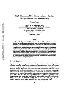
√ Figure 1: Illustrative example: i.i.d. Gaussian ensemble; p = 256, n = 72, s = 8, and σ = s/3. (a) compare with the Lasso estimator βe which minimizes ℓ2 loss. Here βe has only 3 FPs, but ρ2 is large with a value of 64.73. (b) Compare with the βinit obtained using λn . The dotted lines show the thresholding level t0 . The βinit has 15 FPs, all of which were cut after the 1st step; resulting ρ2 = 12.73. After refitting with b ρ2 is further reduced to 0.51. OLS in the 2nd step, for the β,

6.1 Discussions

Compared to Theorem 1.1, we now put a lower bound on βmin,A0 rather than on the entire set S in Theorem 6.3, with the hope to recover A0 . Choosing the set A0 is rather arbitrary; one could for example, consider the set of variables that are strictly above λσ/2 for instance. Bounds on khA0 k∞ are in general harder to obtain than khA0 k2 ; Under stronger incoherence conditions, such bounds can be obtained; see for example Cand`es and Plan (2009); Lounici (2008); Wainwright (2009b). In general, we can still hope to bound khA0 k∞ by khA0 k2 . Having a tight bound on khT0 k2 (or khT0 k∞ ) and khT0c k2 naturally helps relaxing the requirement on βmin,A0 for Lemma 6.2, while in Lemma 6.1, such tight upper bounds will help us to control both the size of I and kβD k and therefore achieve a tight bound on the ℓ2 loss in the expression of Lemma 4.3. In general, when the strong signals are close to each other in their strength, then a small βmin,A0 implies that we are in a situation with low signal to noise ratio (low SNR); one needs to carefully tradeoff false positives with false negatives; this is shown in our experimental results in Section 7. We refer to Wainwright (2009a) and references therein for discussions on information theoretic limits on sparse recovery where the particular estimator is not specified.

7 Numerical experiments In this section, we present results from numerical simulations designed to validate the theoretical analysis presented in previous sections. In our Thresholded Lasso implementation (we plan to release the imple-

18

mentation as an R package), we use a Two-step procedure as described in Section 1: we use the Lasso as the initial estimator, and OLS in the second step after thresholding. Specifically, we carry out the Lasso using procedure LARS(Y, X) that implements the LARS algorithm Efron et al. (2004) to calculate the full regularization path. We then use λn , whose expression is fixed throughout the experiments as follows, p (7.1) λn = 0.69λσ, where λ = 2 log p/n, in (1.2) to select a βinit from this output path as our initial estimator. We then threshold the βinit using a value t0 typically chosen between 0.5λσ and λσ. See each experiment for the actual value used. Given that columns √ of X being normalized to have ℓ2 norm n, for each input parameter β, we compute its SNR as follows: SN R := kβk22 /σ 2 . b we use metrics defined in Table 1; we also compute the ratio between squared ℓ2 error and To evaluate β, the ideal mean squared error, known as the ρ2 ; see Section 7.3 for details.

7.1 Illustrative example In the first example, we run the following experiment with a setup similar to what was used in Cand`es and Tao (2007) to conceptually compare the behavior of the Thresholded Lasso with the Gauss-Dantzig selector: 1. Generate an i.i.d. Gaussian ensemble Xn×p , where Xij ∼ N (0, 1) are independent, which is then √ normalized to have column ℓ2 -norm n. 2. Select a support set S of size |S| = s uniformly at random, and sample a vector β with independent and identically distributed entries on S as follows, βi = µi (1 + |gi |), where µi = ±1 with probability 1/2 and gi ∼ N (0, 1). 3. Compute Y = Xβ + ǫ, where the noise ǫ ∼ N (0, σ 2 In ) is generated with In being the n × n identity matrix. Then feed Y and X to the Thresholded Lasso with thresholding parameter being t0 to recover b β using β.

√ In Figure 1, we set p = 256, n = 72, s = 8, σ = s/3 and t0 = λσ. We compare the Thresholded Lasso estimator βb with the Lasso, where the full LARS regularization path is searched to find the optimal βe that has the minimum ℓ2 error.

7.2 Type I/II errors We now evaluate the Thresholded Lasso estimator by comparing Type I/II errors under different values of t0 and SNR. We consider Gaussian random matrices for the design X with both diagonal and Toeplitz covariance. We refer to the former as i.i.d. Gaussian ensemble and the latter as Toeplitz ensemble. In the Toeplitz case, the covariance is given by T (γ)i,j = γ |i−j| where 0 < γ < 1. We run under two noise levels: √ √ σ = s/3 and σ = s. For each σ, we vary the threshold t0 from 0.01λσ to 1.5λσ. For each σ and t0 19

combination, we run the following experiment: First we generate X as in Step 1 above. After obtaining X, we keep it fixed and then repeat Steps 2 − 3 for 200 times with a new β and ǫ generated each time and we b We compute the average at the end of 200 runs, which will count the number of Type I and II errors in β. correspond to one data point on the curves in Figure 2 (a) and (b). √ For both types of designs, similar behaviors are observed. For σ = s/3, FNs increase slowly; hence there is a wide range of values from which t0 can be chosen such that FNs and FPs are both zero. In contrast, √ when σ = s, FNs increase rather quickly as t0 increases due to the low SNR. It is clear that the low SNR and high correlation combination makes it the most challenging situation for variable selection, as predicted by our theoretical analysis and others. See discussions in Section 6. In (c) and (d), we run additional experiments for the low SNR case for Toeplitz ensembles. The performance is improved by increasing the sample size or lowering the correlation factor. Table 1: Metrics for evaluating βb Metric Definition Type I errors or False Positives (FPs) # of incorrectly selected non-zeros in βb Type II errors or False Negatives (FNs) # of non-zeros in β that are not selected in βb # of correctly selected non-zeros True positives (TPs) True Negatives (TNs) # of zeros in βb that are also zero in β F P R = F P/(F P + T N ) = F P/(p − s) False Positive Rate (FPR) True Positive Rate (TPR) T P R = T P/(T P + F N ) = T P/s

7.3 ℓ2 loss We now compare the performance of the Thresholded Lasso with the ordinary Lasso by examining the metric ρ2 defined as follows: Pp b (βi − βi )2 2 ρ = Pp i=1 . 2 2 i=1 min(βi , σ /n)

We first run the above experiment using i.i.d. Gaussian ensemble under the following thresholds: t0 = √ √ λσ for σ = s/3, and t0 = 0.36λσ for σ = s. These are chosen based on the desire to have low errors of both types (as shown in Figure 2 (a)). Naturally, for low SNR cases, small t0 will reduce Type II errors. In practice, we suggest using cross-validations to choose the exact constants in front of λσ. We plot the histograms of ρ2 in Figure 2 (e) and (f). In (e), the mean and median are 1.45 and 1.01 for the Thresholded Lasso, and 46.97 and 41.12 for the Lasso. In (f), the corresponding values are 7.26 and 6.60 for the Thresholded Lasso and 10.50 and 10.01 for the Lasso. With high SNR, the Thresholded Lasso performs extremely well; with low SNR, the improvement of the Thresholded Lasso over the ordinary Lasso is less prominent; this is in close correspondence with the Gauss-Dantzig selector’s behavior as shown by Cand`es and Tao (2007). Next we run the above experiment under different sparsity values of s. We again use i.i.d. Gaussian ensemble 20

i.i.d. Gaussian; Type I/II errors

Toeplitz; Type I/II errors s/3 γ= 0.9 n = 72 Type I s/3 γ= 0.9 n = 72 Type II s γ= 0.9 n = 72 Type I s γ= 0.9 n = 72 Type II

Value

10 0

5

10 0

5

Value

σ= σ= σ= σ=

20

n = 72 Type I n = 72 Type II n = 72 Type I n = 72 Type II

15

s/3 s/3 s s

15

20

σ= σ= σ= σ=

0.0

0.5

1.0

1.5

0.0

0.5

Threshold

(a)

Toeplitz; Type I/II errors (σ= s)

0

0

5

10

Value

15

20

γ= 0.9 n = 72 Type I γ= 0.9 n = 72 Type II γ= 0.5 n = 72 Type I γ= 0.5 n = 72 Type II

10

15

20

γ= 0.9 n = 72 Type I γ= 0.9 n = 72 Type II γ= 0.9 n = 144 Type I γ= 0.9 n = 144 Type II γ= 0.9 n = 288 Type I γ= 0.9 n = 288 Type II

5

Value

1.5

(b)

Toeplitz; Type I/II errors (σ= s)

0.0

0.5

1.0

1.5

0.0

0.5

Threshold

1.5

(d) i.i.d. Gaussian; Histogram of ρ2 (σ= s) 40

i.i.d. Gaussian; Histogram of ρ2 (σ= s/3)

250

1.0 Threshold

(c)

n = 72 Thresholded Lasso n = 72 Lasso

20 10

100

Frequency

150

30

200

n = 72 Thresholded Lasso n = 72 Lasso

0

0

50

Frequency

1.0 Threshold

0

50

100 ρ2

150

200

0

(e)

5

10

15 ρ2

20

25

30

(f)

Figure 2: p = 256 s = 8. (a) (b) Type I/II errors for i.i.d. Gaussian and Toeplitz ensembles. Each vertical bar represents ±1 std. The unit of x-axis is in λσ. For both types of design matrices, FPs decrease and FNs increase as the threshold increases. For Toeplitz ensembles, in (c) with fixed correlation γ, FNs decrease with more samples, and in (d) with fixed sample size, FNs decrease as the correlation γ decreases. (e) (f) Histograms of ρ2 under i.i.d Gaussian ensembles from 500 runs. 21

√ with p = 2000, n = 400, and σ = s/3. The threshold is set at t0 = λσ. The SNR for different s is fixed at around 32.36. Table 2 shows the mean of the ρ2 for the Lasso and the Thresholded Lasso estimators. The Thresholded Lasso performs consistently better than the ordinary Lasso until about s = 80, after which both break down. For the Lasso, we always choose from the full regularization path the optimal βe that has the minimum ℓ2 loss. Table 2: ρ2 under different sparsity and fixed SNR. Average over 100 runs for each s. s 5 18 20 40 60 80 100 SNR 34.66 32.99 32.29 32.08 32.28 32.56 32.54 Lasso 17.42 22.01 44.89 52.68 31.88 29.40 47.63 Thresholded Lasso 1.02 0.96 1.11 1.54 10.32 29.38 53.81

7.4 Linear Sparsity We next present results demonstrating that the Thresholded Lasso recovers a sparse model using a small number of samples per non-zero component in β when X is a subgaussian ensemble. We run under three cases of p = 256, 512, 1024; for each p, we increase the sparsity s by roughly equal steps from s = 0.2p/log(0.2p) to p/4. For each p and s, we run with different sample size n. For each tuple (n, p, s), we run an experiment similar to the one described in Section 7.2 with an i.i.d. Gaussian ensemble X being fixed while repeating Steps 2 − 3 100 times. In Step 2, each randomly selected non-zero coordinate of β is assigned a value of ±0.9 with probability 1/2. After each run, we compare βb with the true β; if all components match in signs, we count this experiment as a success. At the end of the 100 runs, we compute the percentage of successful runs as the probability of success. We compare with the ordinary Lasso, for which we search over the full regularization path of LARS and choose the β˘ that best matches β in terms of support. q √ We experiment with σ = 1 and σ = s/3. For σ = 1, we set t0 = ft |Sb0 |λσ, where Sb0 = {j : βj,init ≥ 0.5λn = 0.35λσ} √ for λn as in (7.1), and ft is chosen from the range of [0.12, 0.24] (cf. Section 3). For σ = s/3, we set t0 = 0.7λσ with SNR being fixed. The results are shown in Figure 3. We observe that under both noise levels, the Thresholded Lasso estimator requires much fewer samples than the ordinary lasso in order to conduct exact recovery of the sparsity pattern of the true linear model when all non-zero components are sufficiently large. When σ is fixed as s increases, the SNR is increasing; the experimental results illustrate the behavior of sparse recovery when it is close to the noiseless setting. Given the same sparsity, more samples are required for the low SNR case to reach the same level of success rate. Similar behavior was also observed for Toeplitz and Bernoulli ensembles with i.i.d. ±1 entries.

7.5 ROC comparison We now compare the performance of the Thresholded Lasso estimator with the Lasso and the Adaptive Lasso by examining their ROC curves. Our parameters are p = 512, n = 330, s = 64 and we run under 22

1.0 0.8 0.6

s = 8 Thresholded Lasso s = 8 Lasso s = 32 Thresholded Lasso s = 32 Lasso

0.0

0.0

0.2

0.4

0.6

Prob. of success

0.8

s = 8 Thresholded Lasso s = 8 Lasso s = 64 Thresholded Lasso s = 64 Lasso

0.2

Prob. of success

p = 512 σ = s/3

0.4

1.0

p = 256 σ = 1

20

50

100

200 n

500

1000

0

200

400 n

(a)

1.0 0.8 0.6 0.4

s=8 s=18 s=32 s=48

0.0

0.0

Prob. of success

0.4

s=18 s=36 s=64 s=103 s=128 s=192 s=256

0.2

0.6

0.8

1.0

p = 512 σ = s/3

0.2

Prob. of success

800

(b)

p = 1024 σ = 1

200

400

600

800

0

100

200

n

(c)

300 n

400

500

600

(d)

p = 1024 σ = s/3

400

0.4

n 600

0.6

800

0.8

1000

1.0

p = 1024 Sample size vs. Sparsity

Prob. of success 90% σ= 1 80% σ= 1 90% σ= s/3 80% σ= s/3

0.0

200

s=18 s=36 s=64 s=96

0.2

Prob. of success

600

0

200

400

600 n

(e)

800

1000

1200

0

50

100

150 s

200

250

300

(f)

Figure 3: (a) (b) Compare the probability of success for p = 256 and p = 512 under two noise levels. The Thresholded Lasso estimator requires much fewer samples than the ordinary Lasso. (c) (d) (e) show the probability of success of the Thresholded Lasso under different levels of sparsity and noise levels when n increases for p = 512 and 1024. (f) The number of samples n increases almost linearly with s for p = 1024. √ More samples are required to achieve the same level of success when σ = s/3 due to the relatively low SNR. 23

i.i.d. Gaussian; ROC Comparison ( σ= s)

TPR

0.4

0.4

TPR

0.6

0.6

0.8

0.8

1.0

1.0

i.i.d. Gaussian; ROC Comparison ( σ= s/3)

0.2

Lasso Adaptive Lasso Thresholded Lasso

0.0

0.0

0.2

Lasso Adaptive Lasso Thresholded Lasso

0.00

0.05

0.10

0.15

0.00

FPR

0.05

0.10

0.15

FPR

(a)

(b)

Figure 4: p = 512 n = 330 s = 64. ROC for the Thresholded Lasso, ordinary Lasso and Adaptive Lasso. The Thresholded Lasso clearly outperforms the ordinary Lasso and the Adaptive Lasso for both high and low SNRs. √ √ two cases: σ = s/3 and σ = s. In the Thresholded Lasso, we vary the threshold level from 0.01λσ to 1.5λσ. For each threshold, we run the experiment described in Section 7.2 with an i.i.d. Gaussian ensemble b X being fixed while repeating Steps 2− 3 100 times. After each run, we compute the FPR and TPR of the β, and compute their averages after 100 runs as the FPR and TPR for this threshold. For the Lasso, we compute the FPR and TPR for each output vector along its entire regularization path. For the Adaptive Lasso, we use the optimal output βe in terms of ℓ2 loss from the initial Lasso penalization path as the input to its second step, that is, we set βinit := βe and use wj = 1/βinit,j to compute the weights for penalizing those non-zero components in βinit in the second step, while all zero components of βinit are now removed. We then compute the FPR and TPR for each vector that we obtain from the second step’s LARS output. We implement the algorithms as given in Zou (2006), the details of which are omitted here as its implementation has become standard. The ROC curves are plotted in Figure 4. The Thresholded Lasso performs better than both the ordinary Lasso and the Adaptive Lasso; its advantage is more apparent when the SNR is high.

8 Conclusion In this paper, we show that the thresholding method is effective in variable selection and accurate in statistical estimation. It improves the ordinary Lasso in significant ways. For example, we allow very significant number of non-zero elements in the true parameter, for which the ordinary Lasso would have failed. On the theoretical side, we show that if X obeys the RE condition and if the true parameter is sufficiently sparse, the Thresholded Lasso achieves the ℓ2 loss within a logarithmic factor of the ideal mean square error one would achieve with an oracle, while selecting a sufficiently sparse model I. This is accomplished when p √ threshold level is at about 2 log p/nσ, assuming that columns of X have ℓ2 norm n. We also report a similar result on the Gauss-Dantzig selector under the UUP, built upon results from Cand`es and Tao (2007). 24

When the SNR is high, almost exact recovery of the non-zeros in β is possible as shown in our theory; exact recovery of the support of β is shown in our simulation study when n is only linear in s for several Gaussian and Bernoulli random ensembles. When the SNR is relatively low, the inference task is difficult for any estimator. In this case, we show that Thresholded Lasso tradeoffs Type I and II errors nicely: we recommend choosing the thresholding parameter conservatively. Algorithmic issues such as how to get an estimate on σ and parameters related to the incoherence conditions is left as future work. While the current focus is on ℓ2 loss, we are also interested in exploring the sparsity oracle inequalities for the Thresholded Lasso under the RE condition as studied in Bickel et al. (2009) in our future work.

A

Proof of Theorem 1.1

Proving Theorem 1.1 involves showing that the Lasso and the Dantzig selector satisfy (3.2). These have been proved in Bickel et al. (2009). Theorem 1.1 is then an immediate corollary of Theorem 3.1 under assumptions therein. We note that on Ta , it holds that kυinit,S c k1 ≤ k0 kυinit,S k1 , where k0 = 1 for the Dantzig selector when λn ≥ λσ,a,p and k0 = 3 for the Lasso, when λn ≥ 2λσ,a,p for the Lasso. Then on Ta as in (1.15), (3.2) holds with B0 = 4K 2 (s, 3) and B1 = 3K 2 (s, 3) for Lasso under RE(s, 3, X) and (3.2) holds with B0 = B1 = 4K 2 (s, 1) for the Dantzig selector under RE(s, 1, X); See Zhou (2009a) for deriving the exact constants here.

B Proof of Theorem 1.4 Proof of Theorem 1.4. It is clear by construction that under Ta , X βbI = PI Y and |I| ≤ 2s0 . Hence

√

√

b

X βI − Xβ / n = k(PI − Id)Xβ + PI ǫk2 / n 2 √ √ ≤ kXI c βD k2 / n + kPI ǫk2 / n p p |I|(1 + a)Λmax (|I|)λσ ≤ Λmax (s) kβD k2 + Λmin (|I|) p √ where we have on Ta , for λσ,a,p = 1 + aλσ, where λ = 2 log p/n,

√

√

XI (XIT XI )−1 XIT ǫ / n ≤ XI (XIT XI /n)−1 / n XIT ǫ/n 2 2 2 p p p Λmax (|I|) |I|λσ,a,p |I|(1 + a)Λmax (|I|)λσ ≤ ≤ Λmin (|I|) Λmin (|I|) √ Now by Lemma 4.2 and 5.2, we have kβD k2 ≤ C s0 λσ for some constant C.

25

C

Proof of Proposition 1.5

p Recall that |βj | ≤ λσ for all j > a0 as defined in (6.1); hence for λ = 2 log p/n, we have by (G.1), Pp Ps 2 2 2 2 2 2 i>a0 min(βi , λ σ ) = i>a0 βi ≤ (s0 − a0 )λ σ ; hence p {j ∈ Ac0 : |βj | ≥ log p/(c′ n)σ} ≤ 2c′ (s0 − a0 ) where |T0 \ A0 | = s0 − a0 . Now given that βi ≥ βj for all i ∈ T0 , j ∈ T0c , the proposition holds.

D

Proof of Theorem 3.1

We first state two lemmas. Define υinit = βinit − β and υ (i) = βb(i) − β. Lemma D.1. Under assumptions in Theorem 3.1, suppose on Ta ∩ Qb ,



(i) and Γ := max ti . βmin ≥ Ξ + Γ where Ξ := max υS i=0,1

∞

i=0,1

(D.1)

Then S ⊆ Sb2 ⊆ Sb1 .

Proof. We have

S βinit,j ≥ βmin − kυinit,S k∞ ≥ βmin − Ξ ≥ Γ = t0 and

∀j ∈

(1) (1) βb ≥ βmin − υ ≥ βmin −Ξ ≥ Γ ≥ t1 . Thus the lemma holds by definition of Sbi , for i = 0, 1, 2. j

S

∞

The following lemma follows from Lemma 4.3, by plugging in kβD k2 = 0. Lemma D.2. (ℓ2 -loss for the OLS estimators) Suppose that I ⊇ S and |I| ≤ 2s, then the OLS estimator p βbI := (XIT XI )−1 XIT Y satisfies on Ta , kβbI − βk2 ≤ λσ,a,p |I|/Λmin (|I|) which satisfies (3.4) with B2 = 1/(BΛmin (2s)). Proof of Theorem 3.1. It is clear by construction that Sb2 ⊆ Sb1 ⊆ Sb0 .

(D.2)

Recall that Sb0 is obtained by thresholding βinit with 4λn , hence by (3.2), we have |Sb0 \ S| ≤

kυinit,S c k1 B 1 λn s B1 s . ≤ ≤ 4λn 4λn 4

1. If B1 ≤ 4, we have that |Sb0 | ≤ 2s;

2. Otherwise, we have |Sb0 | ≤ s + B1 s/4 ≤ B1 s/2. q Hence for ti = 4λn |Sbi |, ∀i = 0, 1 and Γ as in (D.1), it holds by (D.2) that Γ = t0 = 4λn

q

 p √  √ |Sb0 | ≤ λn s max 2 2B1 , 4 2 . 26

(D.3)

Now given (3.3) and (3.2), we have ∀j ∈ S, βinit,j ≥ βmin − kυinit,S k∞ ≥ βmin − kυinit,S k2 ≥ Γ = t0 ,

√ and hence it holds that S ⊆ Sb1 ⊆ Sb0 by construction of Sb1 , and hence t0 ≥ 4λn s. Now by (3.2), we have for s ≥ B12 /16, √ kυinit,S c k1 B1 s B1 λn s b √ < < s; and |Sb1 | < 2s. (D.4) ≤ |S1 \ S| < t0 4λn s 4 For the OLS estimator βb(1) with I = Sb1 , by Lemma D.2, we have on Ta √ √

√ λσ,a,p s1 λn s 1

b(1) ≤ ≤ B2 λn 2s, where s1 := Sb1

β − β ≤ Λmin (s1 ) BΛmin (2s) 2

where λn ≥ Bλσ,a,p , for λσ,a,p as in (1.15), and B2 = 1/(BΛmin (2s)). Clearly we have by definition of Ξ in (D.1),

√ √

(i) Ξ ≤ max υS ≤ max{B0 , 2B2 }λn s i=0,1

2

and thus βmin ≥ Ξ + Γ holds given (3.3) and (D.3). By Lemma D.1, we have Sb i ⊇ S, ∀i = 0, 1, 2. It remains to show (3.5) and (3.4); Upon thresholding βb(1) with t1 , we have for s1 := Sb1 and λn ≥ Bλσ,a,p ,  2 √

2 λσ,a,p s1 1 1

≤ |Sb2 \ S| ≤ υ (1) /t21 ≤ . · √ Λmin (s1 ) 4λn s1 2 16B 2 Λ2min (s1 )

we have on Ta ∩ Qb by Lemma D.2, Now for the final estimator in (3.1),q



√

b

b(2)

β − β = β − β = λσ,a,p |Sb2 |/Λmin (|Sb2 |) ≤ λn B2 2s. 2

2

E Proofs for the Gauss-Dantzig selector Recall βinit is the solution to the Dantzig selector. We write β = β (1) + β (2) where (1)

βj

(2)

= βj · 11≤j≤s0 and βj

= βj · 1j>s0 .

Let h = βinit −β (1) , where β (1) is hard-thresholded version of β, localized to T0 = {1, . . . , s0 }. Let T1 be the s0 largest positions of h outside of T0 ; Let T01 = T0 ∪ T1 . The proof of Proposition 4.1(cf. Cand`es and Tao (2007)) yields the following: √ khT01 k2 ≤ C0′ λp,τ σ s0 , for C0′ as in (4.1)  

hT c ≤ C1 λp,τ σs0 , where C1 = C0′ + 1 + δ , and 0 1 1−δ−θ



hT c ≤ hT c /√s0 ≤ C1 λp,τ σ √s0 , (cf. Lemma F.2). 01 2 0 1 27

(E.1) (E.2) (E.3)

Proof of Lemma 4.2. Consider the set I ∩ T0c := {j ∈ T0c : |βj,init | > t0 }. It is clear by definition of h = βinit − β (1) and (E.2) that



(E.4) |I ∩ T0c | ≤ βT0c ,init 1 /t0 = hT0c 1 /t0 < s0 ,

where t0 ≥ C1 λp,τ σ. Thus |I| = |I ∩ T0 | + |I ∩ T0c | ≤ 2s0 ; Now (1.16) holds given (E.4) and |I ∪ S| = |S| + |I ∩ S c | ≤ s + |I ∩ T0c | < s + s0 . We now bound kβD k22 . By (E.1) and (6.2), where D11 ⊂ T0 , we √ have for t0 < C4 λp,τ σ s0 , √ kβD k22 ≤ (s0 − a0 )λ2 σ 2 + (t0 s0 + khT0 k2 )2 ≤ ((C4 + C0′ )2 + 1)λ2p,τ σ 2 . Proof of Lemma 4.3. Note that XI c βI c = XSD βSD . We have βbI = (XIT XI )−1 XIT Y = (XIT XI )−1 XIT (XI βI + XI c βI c + ǫ)

= βI + (XIT XI )−1 XIT XSD βSD + (XIT XI )−1 XIT ǫ;



Hence βbI − βI = (XIT XI )−1 XIT XSD βSD + (XIT XI )−1 XIT ǫ 2 2

T

−1 T

≤ (XI XI ) XI XSD βSD 2 + (XIT XI )−1 XIT ǫ 2 ,

where the second term is bounded as Lemma D.2: we have on Ta ,



p

X T X −1

T

|I| XIT ǫ

I I

(XI XI )−1 XIT ǫ ≤

≤ λσ,a,p



2

n n 2 Λmin (|I|)

(E.5)

(E.6)

2

p √ by (1.8), where λσ,a,p = 1 + aλσ for λ = log p/n. We now focus on bounding the first term in (E.5). Let PI denote the orthogonal projection onto I. Let c = (XIT XI )−1 XIT XSD βSD , hence XI c = PI XSD βSD . By the disjointness of I and SD , we have for PI XSD βSD := XI c, kPI XSD βSD k22 = kck2 kPI XSD βSD k2

h PI XSD βSD , XSD βSD i = h XI c, XSD βSD i

≤ nθ|I|,|SD | kck2 kβSD k2 where kPI XSD βSD k2 kXI ck2 ≤ p ; Hence ≤ p nΛmin (|I|) nΛmin (|I|) √ nθ|I|,|SD | kβSD k2 where kβSD k2 = kβD k2 ≤ p Λmin (|I|)

and kck2 ≤ θ|I|,|SD | kβD k2 /Λmin (|I|). Now we have on Ta , by (E.6),





b

βI − βI ≤ (XIT XI )−1 XIT XSD βSD 2 + (XIT XI )−1 XIT ǫ 2 2 p θ|I|,|SD | |I| kβD k2 + λσ,a,p . ≤ Λmin (|I|) Λmin (|I|)

2

2



Now the lemma holds given βbI − β = βbI − βI + kβI − βk22 . 2

2

28

(E.7) (E.8)

Proof of Theorem 1.2. It holds by definition of SD that I ∩ SD = ∅. It is clear by Lemma 4.2 that |SD | < s and |I| ≤ 2s0 and |I ∪ SD | ≤ |I ∪ S| ≤ s + s0 ≤ 2s; Thus for βbI = (XIT XI )−1 XIT Y , we have p for λ = 2 log p/n, and by (4.5) ! 2

2

2θ|I|,|S 2|I|

b 2 D| + 2 λ2

βI − β ≤ kβD k2 1 + 2 2 Λmin (|I|) Λmin (|I|) σ,a,p ! ! 2 √ 2θs,2s 4(1 + a) 0 2 2 −1 2 ′ 2 ≤ λ σ s0 ( 1 + a + τ ) ((C0 + C4 ) + 1) 1 + 2 + 2 . Λmin (2s0 ) Λmin (2s0 ) Thus the theorem holds for C3 as in (4.3) by (4.5), where it holds for τ > 0 that θs,2s0 θs,2s 1 − δ2s − τ ≤ ≤ 0.

F

Oracle properties of the Lasso

We first show Lemma F.1, which gives us the prediction error using βT0 . p Lemma F.1. Suppose that (1.5) holds. We have for λ = (2 log p)/n. p √ √ Λmax (s − s0 )λσ s0 . kXβ − XβT0 k2 / n ≤

(F.1)



√ √ √ Proof. The lemma holds given that βT0c 2 ≤ λσ s0 , and kXβ − XβT0 k2 / n = XβT0c 2 / n ≤

p Λmax (s − s0 ) βT0c 2 .

We then state Lemma F.2, followed by the proof of Theorem 5.1, where we do not focus on obtaining the best constants. Lemma F.2 is the same ( up to normalization) as Lemma 3.1 in Cand`es and Tao (2007). We note that in their original statement, the UUP condition is assumed; a careful examination of their proof shows that it is a sufficient but not necessary condition; indeed we only need to assume that Λmin (2s0 ) > 0 and θs0 ,2s0 < ∞, as we show below. The proof is included by the end of this section for the purpose of a self-complete presentation. Lemma F.2. Suppose Λmin (2s0 ) > 0 and θs0 ,2s0 < ∞. Then

θs0 ,2s0 1

hT c p √ kXhk2 + √ 0 1 s0 Λmin (2s0 ) Λmin (2s0 ) n

2 X

2 ≤ hT0c 1 1/k2 ≤ hT0c 1 /s0 and thus

khT01 k2 ≤

hT c 2 01 2

khk2 ≤

k≥s0 +1

khT01 k22



hT c 2 + s−1 0 0 1

29

Proof of Theorem 5.1. Throughout this proof, we assume that Ta holds. We use βb := βinit to represent b we have the solution to the Lasso estimator in (1.2); By the optimality of β,



2 1 1



(F.2) kY − XβT0 k22 ≤ λn kβT0 k1 − λn βb , where

Y − X βb − 1 2n 2 2n

2

2

2



b T X T ǫ + kǫk2

Y − X βb = Xβ − X βb + ǫ = X βb − Xβ + 2(β − β) 2

2

2

2

and similarly, we have for β0 = βT0 ,

kY − Xβ0 k22 = kXβ − Xβ0 + ǫk22 = kXβ − Xβ0 k22 + 2(β − β0 )T X T ǫ + kǫk22 ;

Let h = βb − β0 . Thus by (F.2) and the triangle inequality, we have on Ta

2

b

X β − Xβ kXβ − Xβ0 k22 2hT X T ǫ 2 ≤ + + 2λn (kβ0 k1 − kh + β0 k1 ) n n n

T

X ǫ

kXβ − Xβ0 k22

+ 2λn (khT k − hT c ) ≤ + 2 khk1 0 1

0 1 n n ∞ 2

kXβ − Xβ0 k2 ≤ + 3λn khT0 k1 − λn hT0c 1 , n where we have used the fact that λn ≥ 2λσ,a,p for a ≥ 0; Thus we have on Ta ,

2



b 2

X β − Xβ /n + λn hT0c 1 ≤ kXβ − Xβ0 k2 /n + 3λn khT0 k1 , 2

(F.3)

which is also the starting point of our analysis on the oracle inequalities of the Lasso estimator. Now we differentiate between two cases. 1. Suppose that on Ta , kXβ − Xβ0 k22 /n ≥ 3λn khT0 k1 . We then have that

2

b

2

X β − Xβ /n + λn hT c ≤ 2 kXβ − Xβ0 k /n 0

2

1

2

and hence for λn = d0 λσ, where d0 ≥ 2, we have by Lemma F.1,

hT c ≤ 2Λmax (s − s0 )λσs0 /d0 ≤ Λmax (s − s0 )λσs0 . 0 1

Now by (F.3), we have

khk1 ≤ kXβ − Xβ0 k22 /(nλn ) + 4 khT0 k1 kXhk2

≤ 7 kXβ − Xβ0 k22 /(3nλn ) ≤ 7Λmax (s − s0 )λσs0 /(3d0 ) and clearly

√

≤ X βb − Xβ + kXβ − Xβ0 k2 ≤ ( 2 + 1) kXβ − Xβ0 k2 . 2

By Lemma F.2, we have on Ta ,

θs0,2s0 1 kXhk2 + √ hT0c 1 √ p Λmin (2s0 ) s0 n Λmin (2s0 ) ! p p θs0 ,2s0 Λmax (s − s0 ) Λmax (s − s0 ) √ √ p ≤ λσ s0 p ( 2 + 1) + Λmin (2s0 ) Λmin (2s0 ) p √ √ Λmax (s − s0 ) θs0 ,2s0 Λmax (s − s0 ) + = Dλσ s0 , for D = ( 2 + 1) p . Λmin (2s0 ) Λmin (2s0 )

khT01 k2 ≤

30

(F.4)

2. Otherwise, suppose on Ta , we have kXβ − Xβ0 k22 /n ≤ 3λn khT0 k1 ; thus

2

b

X β − Xβ /(nλn ) + hT0c 1 ≤ 6 khT0 k1 2

and hT0c 1 ≤ 6 khT0 k1 , which under the RE(s0 , 6, X) condition immediately implies that √ khT0 k2 ≤ K(s0 , 6) kXhk2 / n.

(F.5)

The rest of the proof is devoted to this second case. We use K := K(s0 , 6) as a shorthand below. By (F.3), we have on Ta ,

2

b

2 X β − Xβ

/n + λn hT0c 1 − kXβ − Xβ0 k2 /n 2 √ 3Kλn s0 √ √ kXhk2 (by (F.5)) ≤ 3λn khT0 k1 ≤ 3λn s0 khT0 k2 ≤ n

√ √ √

3Kλn s0 X βb − Xβ + 3Kλn s0 kXβ − Xβ0 k2 / n 2

2

√ √ √

≤ 3Kλn s0 kXβ − Xβ0 k2 / n + X βb − Xβ /n + (3Kλn s0 )2 ,

(F.6)

2

from which the following immediately follows: for λn = d0 λσ ≥ 2λσ,a,p , we have

√

hT c ≤ kXβ − Xβ0 k2 /(nλn ) + 3K √s0 kXβ − Xβ0 k / n + (3K/2)2 λn s0 2 2 0 1 2  p p = kXβ − Xβ0 k2 / nλn + (3K/2) λn s0 := D1′ λσs0

p √ where D1′ = ( Λmax (s − s0 )/d0 +3K(s0 , 6) d0 /2)2 . Similarly, we can derive a bound on khk1 from (F.3); we have on Ta ,

2

b

2

X β − Xβ /n + λn hT0c 1 + λn khT0 k1 − kXβ − Xβ0 k2 /n ≤ 4λn khT0 k1 2 √ √ √ ≤ 4 λn s0 khT0 k2 ≤ 4Kλn s0 kXhk2 / n (by (F.5))

2 √ √ √

≤ 4Kλn s0 kXβ − Xβ0 k2 / n + X βb − Xβ /n + (2Kλn s0 )2 2

Hence it is clear that for λn = d0 λσ ≥ 2λσ,a,p , we have by Lemma F.2, on Ta ,

√ √ khk1 ≤ kXβ − Xβ0 k22 /(nλn ) + 4K s0 kXβ − Xβ0 k2 / n + 4K 2 λn s0 2  p p = kXβ − Xβ0 k2 / nλn + 2K λn s0 = D2 λσs0

2 p √

where D2 = ( Λmax (s − s0 )/d0 + 2K(s0 , 6) d0 )2 . Now we derive a bound for X βb − Xβ /n; our 2 √ starting point is (F.6), from which by shifting items around and adding (3Kλn s0 )2 to both sides, we obtain

2

√

√ √

b

b

X β − Xβ /n − 3Kλn s0 X β − Xβ / n + (3Kλn s0 )2 + λn hT0c 1 2 2 √ √ √ 2 ≤ kXβ − Xβ0 k2 /n + 3Kλn s0 kXβ − Xβ0 k2 / n + (3Kλn s0 /2)2 31

Thus we have for λn = d0 λσ ≥ 2λσ,a,p ,  √ 


2 √ 3Kλn s0 2 √ 1

√ X βb − Xβ − + λn hT0c 1 ≤ kXβ − Xβ0 k2 / n + 3Kλn s0 /2 n 2 2 and hence

√

√ √

b

X β − Xβ / n ≤ kXβ − Xβ0 k2 / n + 3Kλn s0 2  √ p ≤ λσ s0 Λmax (s − s0 ) + 3d0 K(s0 , 6) .

(F.7)

by Lemma F.2. Under RE(s0 , 6, X) condition, we have by (F.7)

 √ K(s0 , 6) 

b

khT0 k2 ≤ K(s0 , 6) kXhk2 / n ≤ √

X β − Xβ + kXβ − Xβ0 k2 2 n √ √
≤ K(s0 , 6) 2 kXβ − Xβ0 k2 / n + 3K(s0 , 6)λn s0 p √ ≤ λσ s0 K(s0 , 6)(2 Λmax (s − s0 ) + 3d0 K(s0 , 6)).

Let T1 be the s0 largest positions of h outside of T0 ; Now by a property as derived in Zhou (2009a) (Proposition A.1), we also have for K := K(s0 , 6). p p √ √ khT01 k2 ≤ 2/nK(s0 , 6) kXhk2 ≤ λσ 2s0 K(2 Λmax (s − s0 ) + 3d0 K) ≤ D0 λσ s0 Moreover, we have by Lemma F.2,

2

2

b

b

2 2 2 2 ≤ 2 β − β β − β

T0 + 2 kβ − βT0 k2 ≤ 2 khk2 + 2λ σ s0 2 2

2 ≤ 2(khT01 k22 + hT0c 1 /s0 ) + 2λ2 σ 2 s0 ≤ 2λ2 σ 2 s0 (D02 + D12 + 1)

We note that (5.1) holds given (F.4) and (F.7).

Remark F.3. We could have bounded khT01 k2 for the second case also by Lemma F.2; we take the form here for simplicity. c into hT , . . . , hT Proof of Lemma F.2. Decompose hT01 such that T2 corresponds to locations of 2 K c the s0 largest coefficients of hT01 in absolute values, and T3 corresponds to locations of the next s0 largest c in absolute values, and so on. Let V be the span of columns of Xj , where j ∈ T01 , and coefficients of hT01 PV be the orthogonal projection onto V . Decompose PV Xh: X X PV Xh = PV XhT01 + PV XhTj = XhT01 + PV XhTj , where



PV XhT ≤ j 2

√

nθs0 ,2s0 Λmin (2s0 )

j≥2

j≥2

X



hT and

hT ≤ hT c /√s0 j 2 j 2 0 1 j≥2

see Cand`es and Tao (2007)) for details; Thus we have





X X





PV XhTj kXhT01 k2 = PV Xh − PV XhTj ≤ kPV Xhk2 +

j≥2

j≥2 2 2 √ X



PV XhT ≤ kXhk + p nθs0 ,2s0√ hT c , ≤ kXhk2 + j 2 2 0 1 Λmin (2s0 ) s0 j≥2 32

1 where we used the fact that kPV k2 ≤ 1. Hence the lemma follows given khT01 k2 ≤ √ √ kXhT01 k2 . Λmin (2s0 ) n

For other bounds, the fact that the kth largest value of hT0c obeys hT0c (k) ≤ hT0c 1 /k has been used; see Cand`es and Tao (2007).

G

Proofs for Lemmas in Section 6

p P Let λ = 2 log p/n. By definition of s0 as in (1.14), we have pi=1 min(βi2 , λ2 σ 2 ) ≤ s0 λ2 σ 2 . We write β = β (11) + β (12) + β (2) where (11)

βj

Now it is clear that

P

(12)

= βj · 11≤j≤a0 , βj j≤a0

= βj · 1a0 s0 .

min(βj2 , λ2 σ 2 ) = a0 λ2 σ 2 and hence

2 X

min(βj2 , λ2 σ 2 ) = β (12) + β (2) ≤ (s0 − a0 )λ2 σ 2 .

(G.1)

2

j>a0

(11)

Proof of Lemma 6.1. It is clear for D11 = D ∩ A0 , we have D11 ⊂ A0 ⊂ T0 ⊂ S. Let βD := (βj )j∈A0 ∩D consist of coefficients of β that are above λσ in their absolute values but are dropped as βj,init < t0 . Now by (G.1), we have

2

(11) 2

(11) 2 (12) 2 (2) + β ≤ βD + (s0 − a0 )λ2 σ 2 , kβD k2 ≤ βD + β 2

2

2

where |D11 | ≤ a0 and thus we have by the triangle inequality,



p

(11) (11) β − β ≤ kβ k + β

D11 ,init

D D11 ,init 2 D ≤ t0 |D11 | + khD11 k2 2 2 √ ≤ t0 a0 + khD11 k2 ;

(G.2)

2

Thus (6.2) holds. Now we replace the bound of |D11 | ≤ a0 with |D11 | ≤

(11)

βD ≤ t0 2

which proves (6.3).

khD11 k2 |βmin,A0 −t0 |2

in (G.2) to obtain

khD11 k2 βmin,A0 + khD11 k2 = khD11 k2 βmin,A0 − t0 βmin,A0 − t0

Proof of Lemma 6.2. Suppose Ta ∩ Qc holds. It is clear by the choice of t0 in (6.5) and by (6.4) that mini∈A0 βbi ≥ βmin,A0 − khA0 k∞ ≥ t0 and D11 = ∅. Thus by (6.5), we can bound |I ∩ T0c |, depending on



2 which one is applicable, by |I ∩ T0c | ≤ βT0c ,init 1 /t0 ≤ s˘0 or by |I ∩ T0c | ≤ βT0c ,init 2 /t20 ≤ s˘0 . Moreover,

2

2 the bounds on βbI − β follows immediately from Lemma 4.3, on event Ta , where θ|I|,|S is bounded in D| 2

Lemma 5.4 given |I| + |SD | ≤ s + |I ∩ T0c | ≤ s + s˘0 ≤ 2s.

Acknowledgment. The author thanks Larry Wasserman and Peter B¨uhlmann for helpful discussions at the early stage of this work, and Sara van de Geer for her positive feedback when I presented this work in the Workshop of the DFG-SNF Research Group at University of Bern, in September 2009. The author would like to thank the NIPS 2009 reviewers for their constructive comments, and John Lafferty and Jun Gao for their encouragements and support. 33

References A DAMCZAK , R., L ITVAK , A. E., , PAJOR , A. and T OMCZAK -JAEGERMANN , N. (2009). Restricted isometry property of matrices with independent columns and neighborly polytopes by random sampling. 0904.4723v1. BARANIUK , R. G., DAVENPORT, M., D E VORE , R. A. and WAKIN , M. B. (2008). A simple proof of the restricted isometry property for random matrices. Constructive Approximation 28 253–263. BARRON , A., B IRGE , L. and M ASSART, P. (1999). Risk bounds for model selection via penalization. Probability Theory and Related Fields 113 301–413. B ICKEL , P. J., R ITOV, Y. and T SYBAKOV, A. B. (2009). Simultaneous analysis of Lasso and Dantzig selector. The Annals of Statistics 37 1705–1732. B IRGE , L. and M ASSART, P. (1997). From model selection to adaptive estimation. In Festschrift for Lucien Le Cam. B IRGE , L. and M ASSART, P. (2001). Gaussian model selection. J. Eur. Math. Soc. (JEMS) 3 203–268. B UNEA , F., T SYBAKOV, A. and W EGKAMP, M. (2007a). Aggregation for gaussian regression. Annals of Statistics 35 1674–1697. B UNEA , F., T SYBAKOV, A. and W EGKAMP, M. (2007b). Sparse density estimation with ℓ1 penalties. In Proceedings of the 20th Annual Conference on Computational Learning Theory (COLT’07). B UNEA , F., T SYBAKOV, A. and W EGKAMP, M. (2007c). Sparsity oracle inequalities for the Lasso. The Electronic Journal of Statistics 1 169–194. C AI , T., WANG , L. and X U , G. (2009). Stable recovery of sparse signals and an oracle inequality. Tech. rep., Department of Statistics, The Wharton School, University of Pennsylvania. C AND E` S , E. and P LAN , Y. (2009). Near-ideal model selection by .1 minimization. Annals of Statistics 37 2145–2177. C AND E` S , E., ROMBERG , J. and TAO , T. (2006). Stable signal recovery from incomplete and inaccurate measurements. Communications in Pure and Applied Mathematics 59 1207–1223. C AND E` S , E. and TAO , T. (2005). Decoding by Linear Programming. IEEE Trans. Info. Theory 51 4203– 4215. C AND E` S , E. and TAO , T. (2006). Near optimal signal recovery from random projections: Universal encoding strategies? IEEE Trans. Info. Theory 52 5406–5425. C AND E` S , E. and TAO , T. (2007). The Dantzig selector: statistical estimation when p is much larger than n. Annals of Statistics 35 2313–2351.

34

C HEN , S. S., D ONOHO , D. L. and S AUNDERS , M. A. (1998). Atomic decomposition by basis pursuit. SIAM Journal on Scientific and Statistical Computing 20 33–61. D ONOHO , D. (2006a). Compressed sensing. IEEE Trans. Info. Theory 52 1289–1306. D ONOHO , D. (2006b). For most large underdetermined systems of equations, the minimal ℓ1 -norm solution is also the sparsest solution. Communications in Pure and Applied Mathematics 59 797–829. D ONOHO , D. L. and J OHNSTONE , I. M. (1994). Ideal spatial adaptation by wavelet shrinkage. Biometrika 81 425–455. E FRON , B., H ASTIE , T., J OHNSTONE , I. and T IBSHIRANI , R. (2004). Least angle regression. Annals of Statistics 32 407–499. F OSTER , D. and G EORGE , E. (1994). The risk inflation criterion for multiple regression. Ann. Statist. 22 1947–1975. G REENSHTEIN , E. and R ITOV, Y. (2004). Persistency in high dimensional linear predictor-selection and the virtue of over-parametrization. Bernoulli 10 971–988. H UANG , J., M A , S. and Z HANG , C.-H. (2008). Adaptive Lasso for sparse high-dimensional regression models. Statist. Sinica 18 1603–1618. KOLTCHINSKII , V. (2009a). Dantzig selector and sparsity oracle inequalities. Bernoulli 15 799–828. KOLTCHINSKII , V. (2009b). Sparsity in penalized empirical risk minimization. Ann. Inst. H. Poincare Probab. Statist. 45 7–57. L OUNICI , K. (2008). Sup-norm convergence rate and sign concentration property of Lasso and Dantzig estimators. Electronic Journal of Statistics 2 90–102. ¨ M EINSHAUSEN , N. and B UHLMANN , P. (2006). High dimensional graphs and variable selection with the Lasso. Annals of Statistics 34 1436–1462. M EINSHAUSEN , N. and Y U , B. (2009). Lasso-type recovery of sparse representations for high-dimensional data. Annals of Statistics 37 246–270. M ENDELSON , S., PAJOR , A. and T OMCZAK -JAEGERMANN , N. (2008). Uniform uncertainty principle for bernoulli and subgaussian ensembles. Constructive Approximation 28 277–289. N EEDELL , D. and T ROPP, J. A. (2008). CoSaMP: Iterative signal recovery from incomplete and inaccurate samples. Applied and Computational Harmonic Analysis 26 301–321. N EEDELL , D. and V ERSHYNIN , R. (2009). Signal recovery from incomplete and inaccurate measurements via regularized orthogonal matching pursuit. IEEE Journal of Selected Topics in Signal Processing, to appear .

35

R ASKUTTI , G., WAINWRIGHT, M. and Y U , B. (2009). Minimax rates of estimation for high-dimensional linear regression over ℓq -balls. In Allerton Conference on Control, Communication and Computer. Longer version in arXiv:0910.2042v1.pdf. R AVIKUMAR , P., WAINWRIGHT, M. and L AFFERTY, J. (2008). High-dimensional ising model selection using ℓ1 -regularized logistic regression. Annals of Statistics To appear; Also in Technical Report 750, Department of Statistics, U.C. Berkeley. RUDELSON , M. and V ERSHYNIN , R. (2006). Sparse reconstruction by convex relaxation: Fourier and gaussian measurements. In 40th Annual Conference on Information Sciences and Systems (CISS 2006). S ZAREK , S. (1991). Condition numbers of random matrices. J. Complexity 7 131–148. T IBSHIRANI , R. (1996). Regression shrinkage and selection via the Lasso. J. Roy. Statist. Soc. Ser. B 58 267–288. G EER , S. and B UHLMANN , P. (2009). On the conditions used to prove oracle results for the lasso. Electronic Journal of Statistics 3 1360–1392.

VAN DE

¨ G EER , S., B UHLMANN , P. and Z HOU , S. (2010). Prediction and variable selection with the adaptive lasso. ArXiv:1001.5176v1.pdf.

VAN DE

G EER , S. A. (2008). High-dimensional generalized linear models and the Lasso. The Annals of Statistics 36 614–645.

VAN DE

WAINWRIGHT, M. (2009a). Information-theoretic limitations on sparsity recovery in the high-dimensional and noisy setting. IEEE Trans. Inform. Theory 55 5728–5741. WAINWRIGHT, M. (2009b). Sharp thresholds for high-dimensional and noisy sparsity recovery using ℓ1 constrained quadratic programming. IEEE Trans. Inform. Theory 55 2183–2202. WASSERMAN , L. and ROEDER , K. (2009). High dimensional variable selection. The Annals of Statistics 37 2178–2201. Z HANG , C.-H. and H UANG , J. (2008). The sparsity and bias of the lasso selection in high-dimensional linear regression. Annals of Statistics 36 1567–1594. Z HANG , T. (2009). Some sharp performance bounds for least squares regression with ℓ1 regularization. Annals of Statistics 37 2109–2144. Z HAO , P. and Y U , B. (2006). On model selection consistency of Lasso. Journal of Machine Learning Research 7 2541–2567. Z HOU , S. (2009a). Restricted eigenvalue conditions on subgaussian random matrices. ArXiv:0904.4723v2. Z HOU , S. (2009b). Thresholding procedures for high dimensional variable selection and statistical estimation. In Advances in Neural Information Processing Systems 22. MIT Press.

36

¨ Z HOU , S., VAN DE G EER , S. and B UHLMANN , P. (2009). Adaptive Lasso for high dimensional regression and gaussian graphical modeling. ArXiv:0903.2515. Z OU , H. (2006). The adaptive Lasso and its oracle properties. Journal of the American Statistical Association 101 1418–1429.

37