forms with custom application-specific accelerators to programmable multi pro- ... in many embedded application domains, such as digital television, multimedia.
Throughput constraint for Synchronous Data Flow Graphs Alessio Bonfietti, Michele Lombardi, Michela Milano, and Luca Benini DEIS, University of Bologna V.le Risorgimento 2, 40136, Bologna, Italy
Abstract. Stream (data-flow) computing is considered an effective paradigm for parallel programming of high-end multi-core architectures for embedded applications (networking, multimedia, wireless communication). Our work addresses a key step in stream programming for embedded multicores, namely, the efficient mapping of a synchronous data-flow graph (SDFG) onto a multi-core platform subject to a minimum throughput requirement. This problem has been extensively studied in the past, and its complexity has lead researches to develop incomplete algorithms which cannot exclude false negatives. We developed a CP-based complete algorithm based on a new throughput-bounding constraint. The algorithm has been tested on a number of non-trivial SDFG mapping problems with promising results.
1
Introduction
The transition in high-performance embedded computing from single CPU platforms with custom application-specific accelerators to programmable multi processor systems-on-chip (MPSoCs) is now a widely acknowledged fact [3, 4]. All leading hardware platform providers in high-volume applications areas such as networking, multimedia, high-definition digital TV and wireless base stations are now marketing MPSoC platforms with ten or more cores and are rapidly moving towards the hundred-cores landmark [5–7]. Large-scale parallel programming has therefore become a pivotal challenge well beyond the small-volume market of high-performance scientific computing. Virtually all key markets in data-intensive embedded computing are in desperate need of expressive programming abstractions and tools enabling programmers to take advantage of MPSoC architectures, while at the same time boosting productivity. Stream computing based on a data-flow model of computation [8, 9] is viewed by many as one of the most promising programming paradigms for embedded multi-core computing. It matches well the data-processing dominated nature of many algorithms in the embedded computing domains of interest. It also offers convenient abstractions (synchronous data-flow graphs) that are at the same time understandable and manageable by programmers and amenable to automatic translation into efficient parallel executions on MPSoC target platforms. Our work addresses one of the key challenges in the development of programming tool-flow for stream computing, namely, the efficient mapping of synchronous
2
data-flow graphs (SDFG) onto multi-core platforms. More in detail, our objective is to find allocations and schedules of SDFG nodes (also called actors or tasks) onto processors that meet throughput constraints or maximize throughput, which can be informally defined as the number of executions of a SDFG in a time unit. In particular, an allocation is an unique association between actors and processors and a schedule is a static order between actors running on the same processor. Meeting a throughput constraint is often the key requirement in many embedded application domains, such as digital television, multimedia streaming, etc. The problem of SDFG mapping onto multiple processors has been studied extensively in the past. However, the complex execution semantic of SDFGs on multiple processors has lead researchers to focus only on incomplete mapping algorithms based on decomposition [12] [14]. Allocation of actors onto processors is first obtained, using approximate cost functions such as workload balancing [12], and incomplete search algorithms. Then the throughput-feasible or throughputmaximal scheduling of actors on single processors is computed, using incomplete search techniques such as list scheduling [8]. The reason for the use of incomplete approaches is that both computing an optimal allocation and an optimal schedule is NP-hard. Our approach is based on Constraint Programming and tackles the overall problem of allocating actors to processors and schedule their order such that a throughput constraint is satisfied; hence we avoid the intrinsic loss of optimality due to the decomposition of the problem into two separated stages. In fact, our method is complete, meaning that it is guaranteed to find a feasible or an optimal solution in case it exists. The core of the approach is a novel throughput constraint, based on the computation of the maximum cycle mean over a graph that is modified during search according to allocation and scheduling decisions. To our knowledge this is the first time a throughput constraint is implemented into a CP language. We have evaluated the scalability of our code on three sets of realistic instances: cyclic, acyclic and strongly connected graphs. The second set of instances is quite difficult and scales poorly, while the first and third sets scale well. We can solve instances up to 20-30 nodes in the order of seconds for finding a feasible solution and in the order of few minutes for proving throughput optimality.
2
Preliminaries on SDFG and HSDFG
Synchronous Dataflow Graphs (SDFGs) [1] are used to model multimedia applications with timing constraints that must be bound to a Multi Processor System on Chip. They allow modeling of both pipelined streaming and cyclic dependencies between tasks. To test the performances of an application on a platform, one important parameter is the throughput. In the following we provide some preliminary notions on synchronous data flow graphs used in this paper. Definition 1. An SDFG is a tuple (A,D) consisting of a finite set A of actors and a finite set D of dependency edges. A dependency edge d = (a,b, p,q,tok)
3
Fig. 1. (A) An example of SDFG; (B) the corresponding equivalent HSDFG
denotes a dependency of actor b on a. When a executes it produces p tokens on d and when b executes it removes q tokens from d. Edge d may also contain initial tokens. This number is notated by tok. Actor execution is defined in terms of firings. An essential property of SDFGs is that every time an actor fires it consumes a given and fixed amount of tokens from its input edges and produces a known and fixed amount of tokens on its output edges. These amounts are called rates. The SDFG illustrated in figure 1A presents initial token on edges (A,A) and (C,B) with tok values respectively 1 and 3. The rates on the edges determine how often actors have to fire w.r.t. each other such that the distribution of tokens over all edges is not changed. This property is captured in the repetition vector. Definition 2. A repetition vector of an SDFG=(A,D) is a function γ : A → N such that for every edge (a, b, p, q, tok) ∈ D from a ∈ A to b ∈ A, pγ(a) = qγ(b). A repetition vector q is called non-trivial if ∀a ∈ A, γ(a) > 0. The SDFG reported in figure 1A has three actors. Actor A has a dependency edge to itself with one token on it. It means that the two firings of A cannot be executed in parallel because the token on the edge (A,A) forces the sequential execution of the actor A. Also, each time A executes it produces one token that can be consumed by B. Each time B executes it produces 3 tokens while C consumes 2 tokens. Also when C executes it produces 2 tokens while C requires 3 tokens to fire. Thus, every 2 executions of B correspond to 3 executions of C. This is captured in the repetition vector reported in figure 1A. Concerning initial tokens, they both define the order of actor firings and the number of instances of a single actor simultaneously running. For example, at the beginning of the application, A only can start (as there are tokens enough on each ingoing arc). A will be then followed by B and then C. An SDFG is called consistent if it has a non-trivial repetition vector. The smallest non-trivial repetition vector of a consistent SDFG is called the repetition vector. Consistency and absence of deadlock are two important properties for SDFGs which can be verified efficiently [2], [11]. Any SDFG which is not consistent requires unbounded memory to execute or deadlocks, meaning that no actor is able to fire. Such SDFGs are not useful in practice. Therefore, we focus on consistent and deadlock free SDFGs.
4
Throughput is an important design constraint for embedded multimedia systems. The throughput of an SDFG refers to how often an actor produces an output token. To compute throughput, a notion of time must be associated with the firing of each actor (i.e., each actor has a duration also called response time) and an execution scheme must be defined. We consider as execution scheme the self timed execution of actors: each actor fires as soon as all of its input data are available (see [11] for details). In a real platform self timed execution is implemented by assigning to each processor a sequence of actors to be fired in fixed order: the exact firing times are determined by synchronizing with other processors at run time. SDFGs in which all rates associated to ports equal 1 are called Homogeneous Synchronous Data Flow Graphs (HSDFGs, [1]). As all rates are 1, the repetition vector for an HSDFG associates 1 to all actors. Every SDFG G = (A,D) can be converted to an equivalent HSDFG GH = (AH,DH), by using the conversion algorithm in [2], sec. 3.8. In figure 1B we report the HSDFG corresponding to the SDFG in figure 1A. For each node in the SDFG we have a number of nodes in the HSDFG equal to the corresponding number in the repetition vector. Equivalence means that there exists a one-to-one mapping between the SDFG and HSDFG actor firings, therefore the two graphs have the same throughput. The fastest method to compute the throughput of an HSDFG is the use of the maximum cycle mean (MCM) algorithm [2], as the throughput is 1/M CM . In the context of SDFGs, the cycle mean of a cycle C is the total computation time of actors in C divided by the number of tokens on the edges in C; the maximum cycle mean for an SDFG is also known as iteration period. Clearly longer cycles influence the throughput more than shorter ones. The problem we face in this paper is the following: given a multiprocessor platform with homogeneous processors we have to allocate each actor to a processor and to order actors on each processors such as all precedence constraints and the throughput constraints are met. Both the allocation and the schedule are static, meaning that they remain the same over all the iterations. In this paper we assume negligible delay associated to inter-processor communication and a uniform memory model for the processors. This models fits well the behavior of a cache-coherent, shared memory single-chip multiprocessor, such as the ARM MPCore [18].
3
Related Work
The body of work on SDFG mapping is extensive and covers more than two decades, starting from the seminal work by Lee and Messerschmitt [10]. Hence, a complete account of all related contributions is not possible in this paper. The interested reader is referred to [2] for an excellent, in-depth survey of the topic. Here we focus on categorizing the two main classes of approaches taken in the past, summarizing state-of-the-art and putting them in perspective with our work.
5
The first class of approaches, pioneered by the group lead by E. Lee [11] and extensively explored by many other researchers [2], can be summarized as follows. A SDFG specification is first checked for consistency, and its nonnull repetition vector is computed. The SDFG is then transformed, using the algorithm described in [2] into a HSDFG. The HSDFG is then mapped onto the target platform in two phases. First, an allocation of HSDFG nodes onto processors is computed, then a static-order schedule is found for each processor. The overall goal is to maximize throughput, given platform constraints. Unfortunately, throughput depends on both allocation and scheduling, but in this approach scheduling decisions are postponed to a second phase. Hence, an approximate cost function is used to drive allocation decisions: for instance, a bin-packing heuristic aiming at balancing processor workload is proposed in [12]. After allocation, scheduling is reduced to a set of single-processor actor ordering decisions. Scheduler implementation issues mandate for static orders, which are decided off-line. This is however not an easy problem to solve either, as throughput depends on the order of execution of actors and we have an exponential blowup of the solution space. Incomplete search strategies are used, such as list scheduling, driven by a priority function related to throughput. For instance, high priority can be given to actors which belong to long cycles in the HSDFG and therefore have most probably more impact on the throughput [2]. The second class of approaches computes mapping and scheduling directly on the SDFG, without a preliminary HSDFG transformation [13]. This has the main advantage to avoid potential blow-up in the number of actors, which can happen for SDFGs with highly un-balanced rates with a large minimum common multiple. Unfortunately, there is no known way to analytically compute throughput for a generic SDFG with scheduling and allocation, hence these approaches resort to heuristic cost functions to generate promising solutions, and then compute the actual throughput by performing state-space exploration on the SDFG with allocation end scheduling information until a fixed point is reached [14]. This process is quite time consuming. Furthermore, even though the throughput computation via state-space exploration is accurate, there is no guarantee that the solutions generated by the heuristic search are optimal. The incomplete approaches summarized above obviously cannot give any proof of optimality. Our work aims at addressing this limitation, and it proposes a complete search strategy which can compute max-throughput mappings for realistic-size instances. Our starting point is a HSDFG, which can be obtained from a SDFG by a pseudo-polynomial transformation. The analysis of complete search strategies starting directly from a generic SDFG, without HSDFG transformation, will be subject of future work.
4
Scheduling and allocation as a Constraint Problem
Due to the cyclic nature of the problem, a scheduling approach deciding the starting time of optional activities running on alternative unary resources has to cope with the transition phase which always appears at execution time be-
6
Fig. 2. The HSDFG corresponding to the SDFG of figure
fore the application becomes periodic (enabling throughput computation). A classical solution is to schedule over time several iterations of the HSDFG until the periodic phase is reached, with a possibly drastical increase of the number of actors. We therefore opted for an alternative approach, somehow similar to Precedence Constraint Posting techniques [20], and devised an order-based, rather than time-based model. Our approach relates to [13] in that the basic idea is to model the effects of design choices by means of modifications to the graph. Consider for example the HSDFG in figure 2A, where all rates are assumed to be one and actors A,D are mapped on one processor, while actors B, C and E on another. From the fact that no more than one task can execute on a processor at the same time, it also follows that two instances of the same task cannot run simultaneously: this can be modeled by adding an auto-cycle to each actor, as depicted in figure 2B where the added arcs are dotted. Moreover, actors mapped on the same processor must be mutually exclusive: this is captured by adding arcs to create a cycle between each pair of non dependent tasks with the same mapping; note this requires adding one arc for the (A, D) and (B, E) pairs in figure 2B and two arcs for the (B, C) and(C, E) pairs. In order to avoid deadlocks a token must be placed for each of these cycles: while the choice is forced for the (A, D) and (B, E) pair, both arcs are suitable for (B, C), (C, E), as hinted by the empty circles in figure 2B. Choosing the placement of those tokens amounts to take scheduling decisions: for example in figure 2C the order B, C, E was chosen. Note the presence of the edge (B,E) is not necessary, since the path from B to E (B,D,E ) implies that the execution of actor E depends on the execution of B. The main advantage with this approach is that a standard throughput computation algorithm can be used (almost) off the shelf to evaluate the effect of each design decision. We therefore devised a two layer CP model; on one level the model features two sets of decision variables, respectively representing the processor each actor is mapped to and the scheduling/ordering decisions, and on another level a set of graph description variables. Let n be the number of actors in the input HSDFG and let p be the number of processor in the platform, then the decision variables are: ∀i = 0 . . . n − 1 : PROCi ∈ [0..p − 1]
∀i = 0 . . . n − 1 : NEXTi ∈ [−1..n − 1]
whereas the (dynamically changing) graph structure is described via a matrix of binary variables Yij ∈ [0, 1] such that Yij = 1 iff an arc from ai to aj ex-
7
ists. Note that the token positioning is implicitly defined by the NEXTi variables and is built on-line only at throughput computation time. The value of NEXTi defines the successor of the actor i; the negative value means the lack of a successor. These variables are connected to allocation decisions and to dependencies between actors. Existing arcs in the input HSDFG result in some pre-filling of the Y matrix, such that Yij = 1 for each arc (ai , aj , 1, 1, tok) in the original graph. Channeling constraints link decision and graph description variables; in particular, as for the PROCi variables, the relation depends on whether a path with no tokens exists in the original graph between two nodes ai , aj . Let us write ai ≺ aj if such path exists; then, if i 6= j and neither ai ≺ aj nor aj ≺ ai : PROCi = PROCj ⇒ Yij + Yji = 2
(1)
Constraint (1) forces two arcs to be added, if two independent nodes are mapped to the same processor (e.g. nodes B and C in figure 2B). If instead there is a path from ai to aj (ai ≺ aj ), then the following constraint is posted: X X (PROCi = PROCj ) ∧ (PROCk = PROCi ) = 0 ∧ (PROCk = PROCj ) = 0 ⇒ Yji = 1 aj ≺ak
ak ≺ai
The above constraint completes dependency cycles: considering only tasks on the same processor (first element in the constraint condition), if there is no task before ai in the original graph (second element) and there is no task after aj in the original graph (third element), then close the loop, by adding an arc from aj to ai . Finally, auto-cycles can be added to each node in a pre-processing step and are not considered here. The NEXT variables do not affect the graph description matrix; a number of constraints, however, are used to ensure their semantic consistence. In first place, dependencies in the input SDFG cannot be violated: thus ai ≺ aj ⇒ NEXTj 6= i. Less intuitively, the presence of an arc (ai , aj , 1, 1, tok) with tok = 1 in an HSDFG implies ai to fire always after aj (e.g. A2 and A1 in fig. 2) , and therefore, NEXTi 6= j. No two nodes can have the same NEXT on the same processor: PROCi = PROCj ⇒ NEXTi 6= NEXTj . Then, a node aj can be next of ai only if they are on the same processor: PROCi 6= PROCj ⇒ NEXTi 6= j. The -1 value is given to the last node of each (non empty) processor: ∀proc :
n−1 X i=0
(PROCi = proc) > 0 ⇒
n−1 X
[(PROCi = proc) × (NEXTi = −1)] = 1
i=0
Finally, transitive closure on the actors running on a single processor is kept by posting a nocycle constraint [19] on the related NEXT variables. Standard tree search is used with minimum size domain as variable selection heuristics. Symmetry due to homogeneous processors are broken at search time.
8
Fig. 3. HSDF graph structure and token positioning for throughput computation during the search; note the number of tokens between actors C and E is overestimated
4.1
Throughput constraint
The relation between decision variables and the throughput value is captured in the proposed model by means of a novel throughput constraint, with signature: th cst(TPUT, [PROCi ], [NEXTi ], [Yij ], W, T ) where TPUT is a real valued variable representing the throughput, [PROCi ], [NEXTi ] and [Yij ] are defined as above, W is a vector of real values such that Wi is the computation time of actor ai and T is a matrix such that Tij is the number of initial tokens tok on the arc from ai to aj . Clearly Tij > 0 implies Yij = 1; note that in this paper we assume Tij = [0, 1]: this is usually true for HSDFG resulting from conversion of an original SDFG. We devised a filtering algorithm consistently updating an upper bound on TPUT (this is sufficient for a throughput maximization problem) and performing what-if propagation on the NEXT and PROC variables. The filtering algorithm relies on throughput computation inspired from the algorithms described in [15] and [16], which in turn are based on Karp’s algorithm (1978). The description is organized in three steps: steps 1 and 2 describe how to build a HSDFG based on current search state to obtain a throughput bound, while step 3 focuses on the computation algorithm. Step 1 - building the input graph: the input for the throughput computation is a “minimal” graph built by adding arcs to the original HSDFG based on current state of the model. More precisely, an arc is assumed to exist between actors ai and aj iff Yij = 1; unbound Y variables are therefore treated as if they were set to 0. Note that the computation of a lower bound for the throughput would require arcs for unbound Y variables as well, thus providing a “maximal” graph. Step 2 - Token positioning: next we construct a dependency graph DG with the same nodes as the original HSDF graph G, and such that an arc (ai , aj ) exists in DG iff either an arc (ai , aj , 1, 1, 0) exists in G (detected since Yij = 1 and Tij = 0) or NEXTi = j. A token matrix T K is then built, according to the following rules: � T Kij = 0 if ai ≺DG aj Yij = 0 ⇒ T Kij = 0 Yij = 1 ⇒ T Kij = 1 otherwise
9
Algorithm 1 Throughput computation - build D table 1: set all Dk (ai ) = −∞, πk (ai ) = N IL, τk (ai ) = 0 2: Vc = {a0 } 3: Vn = ∅ 4: D0 (a0 ) = 0 5: for k = 1 to n do 6: for ai ∈ V do 7: for aj ∈ A+ (ai ) do 8: Vn = Vn ∪ {aj } 9: define T P = max(1, τk (ai ) + T Kij ) 10: define W P = Dk (ai ) + Wj D (a ) W (P ) 11: if T (P ) > τ k(a j) then k j 12: Dk (aj ) = W P, τk (aj ) = T P, πk (aj ) = i 13: end if 14: end for 15: end for 16: find loops on level k 17: Vc = Vn , Vn = ∅ 18: end for
where we write ai ≺DG aj if there is path from ai to aj in DG. This matrix describes the position of the tokens on the new graph G used for the bound computation. The above rules ensure the number of tokens is over-estimated, until all NEXT and PROC are fixed. In the actual implementation, the dependency check is performed without building any graph, while the token matrix T K is actually stored in the constraint. Note that considering a suitable under-estimation of the number of token would be required to compute a throughput lower bound. Figure 3A shows some assignments of decision variables for the HSDFG in figure 2A (remaining variables are considered unbound); figure 3B shows the corresponding arc structure (without autocycles), figure 3C the extracted dependency graph DG and figure 3D the derived token positioning. Step 2: Throughput computation: for a HSDFG, the throughput equals the inverse of a quantity known as the iteration period of the graph and denoted as λ(HSDF G); formally: W (C) 1 = λ(HSDF G) = max C∈HSDF G T (C) th
P where C is a cycle in the HSDFG, W (C)P = ai ∈C Wi is the sum of the execution time of all actors in C and T (C) = (ai ,aj )∈C T Kij is the total number of tokens on the arcs of C. Intuitively, T (C) can be thought of as the amount of concurrency which can be exploited on the cycle. In [15] it is shown how to compute the iteration period as the maximum cycle mean of an opportunely derived delay graph; Karp’s algorithm is used for the computation. With some tricks, we show that a maximum cycle mean algorithm can be used to compute the iteration period directly on a HSDFG. The basic idea is that, according to Karp’s theorem, the critical loop constraining the iteration period can be found by analyzing cycles on the worst case k-arcs paths (e.g. the longest ones) starting from an arbitrary source. Since no cycle can involve more than n nodes, considering k-arcs paths with k up to n
10
Algorithm 2 Throughput computation - finding loops 1: let k be the starting level on the D table 2: let V be the set of nodes to visit on level k 3: for ai ∈ V do 4: define k′ = k, a′ = ai 5: define W C = Wi , T C = 0 6: repeat 7: define h = index of a′ 8: T C = max(1, T C + T Kπ ′ (a′ ),h ) k 9: W C = W C + Wπ ′ (a′ ) k C W C∗ 10: if W T C > T C ∗ then 11: W C = W C∗, T C = T C∗ C∗ 12: TPUT ≤ W T C∗ 13: end if 14: a′ = aπ ′ (a′ ) , k = k − 1 k 15: until a′ = ai ∨ a′ = N IL 16: end for
is sufficient. Our algorithm shares most of its structure with that proposed in [16]. Worst case paths are stored in a (n + 1) × n table D; the element on level (row) k and related to node ai is referred to as Dk (ai ) and contains the length of the k-arcs path P from the source to ai maximizing the quantity W (P )/T (P ) (if any such path exists). Other than D, the algorithm also employs two equally sized tables π and τ , respectively storing the predecessor πk (ai ) of node ai and the number of tokens τk (ai ) on the paths. Pseudo code for the throughput computation is reported in Algorithm 1, where A+ (ai ) denotes the set of direct successors of ai . Once the table is initialized (line 1), an arbitrary source node is chosen; in the current implementation this is the node with minimum index (a0 ). Note that the choice has no influence on the method correctness, but a strong impact on its performance, hence the introduction of a suitable heuristic will be thoroughly considered in the future. Next, the procedure is primed by setting D0 (a0 ) to 0 (line 4) and adding a0 to the list of nodes to visit V (line 3); then we start to fill levels 1 to n one by
Fig. 4. Example of table filling (Algorithm 1)
11
one (lines 6 to 18). For each node in V each successor aj is considered (lines 6, 7), and, if necessary, the corresponding cells in D, π, τ are updated to store the k-arcs path from a0 to aj (lines 9 to 12); in case of an equality at line 11 the number of tokens is considered. Once a level is filled, loops are detected as described in Algorithm 2 and then we move to the next k value (line 17). A single iteration of the algorithm is sufficient to compute the throughput of a strictly connected graph; otherwise, the process is repeated starting from the first never touched node, until no such node exists. Figure 4 shows the value of all tables at each step when Algorithm 1 is executed on the graph of figure 3; all execution times are assumed to be 1. As an example, consider the transition between step 1 and 2 in the figure: at level 1 the set Vc of the nodes to be visited contains actors C and D. When C is visited all its direct successors are processed: when moving from C to B we traverse one more node (W P = D1 (C) + WB = 1 + 1) and collect one more token (T P = τ1 (C) + 1 = 0 + 1), hence we set D2 (B) = W P = 2, τ2 (B) = T P = 1 and the predecessor π2 (B) becomes C; similarly, when processing the arc from C to E, we set D2 (E) = 2, τ2 (E) = 1, π2 (E) = C. Next, actor D is visited; when processing the arc from D to A we set D2 (A) = 2, τ2 (A) = 1, π2 (A) = D; the second outgoing arc of D ends in the already visited node E: for this path W P = 2 and T P = max(1, τ1 (D) + 0) = 1, but no token is collected; for this reason, even if the ratio W P/T P has the same value as D2 (E)/τ2 (E), we set D as the predecessor of E and D2 (E) = 2, τ2 (E) = 0. The loop finding procedure (Algorithm 2) is started at a specific level (let this be k). From each actor ai on level k to be visited, the algorithm moves backward along the predecessor chain (πk′ (a′ ) is the predecessor of current node) collecting execution time of every node met along the path (lines 8, 9). When a second occurrence of the starting node ai is detected (a′ = ai in line 14) a cycle is found. If this loop constrains the iteration period more the last one found so far (line 10), this is set as critical cycle (W C ∗ , T C ∗ — initially W C ∗ = 0, T C ∗ = 1) and pruning is performed (line 12). The algorithm also stops when the start of D is reached (a′ = N IL in line 14). Algorithm 2 is executed for each value of k during the throughput computation. For instance, with regard to figure 4, at step 5 the procedure finds the
proc 2
4
8
nodes 10 15 20 25 10 15 20 25 10 15 20 25
T(opt) T(all) F(all) T(best) 0.03 0.04 53 0.02 0.30(1) 5.27 3658 0.17 2.52(2) 28.37(2) 4374(2) 0.63(2) ------8.33 0.03 0.05 46 0.03 1.13(1) 4.45(1) 3303 0.21 1.94(2) 21.60(2) 1808(2) 0.64(2) ------8.62 0.04 0.06 47 0.03 0.25(1) 4.91(1) 3195 0.20 6.65(2) 26.13(2) 2222(2) 0.72(2) ------9.83
T(worst) T > TL 0.05 0 27.97 1 86.44(2) 2 78.65 3 0.07 0 25.03 1 32.17(2) 2 228.86 3 0.09 0 29.38 1 42.12(2) 2 264.98 3
Table 1. Results for cyclic, connected graphs - times are in seconds
12
loops (stated backward): “A ← D ← B ← E ← D/2 tokens”, “B ← C/1 token”, “D ← A/1 token”, “E ← D ← B/1 token”. No loop is found at this level starting from C. Loop E ← D ← B is critical and sets the iteration bound to 3; the computed throughput is therefore 1/3, which is a valid upper bound for the throughput of the original HSDFG. Note that by finding new loops the upper bound always decreases; hence, if at any step a cycle is found such that the resulting throughput is lower the than the minimum value of the TPUT variable, then the constraint fails. Moreover, it could be proven that no more than 1 token can be collected by traversing a sequence of nodes on a single processor: the filtering algorithm exploits this property to improve the computed bound at early stages of the search, where the number of tokens is strongly overestimated.
5
Experimental Results
The system described so far was implemented on top of ILOG Solver 6.3 and tested on graphs belonging to three distinct classes of HSDFGs, built by means of the generator provided in the SDF3 framework [17]. Graph classes include in first place cyclic, connected graphs, which commonly arise when modeling streaming applications. Those are probably the most interesting instances, as they also reflect the typical structure of homogeneous graphs resulting from the conversion of a SDFG. Note the throughput for a cyclic graph is intrinsically bounded by the heaviest cycle, no matter how many processor it is mapped to. Furthermore, acyclic and strictly connected HSDFGs were considered. Acyclic graphs expose the highest parallelism: this makes them the most challenging instances, but also lets the solver achieve the best throughput values, as no intrinsic bound is present (beside the computation time of the heaviest actor). The class of strictly connected graphs is interesting as this is the type of graph the Maximum Cycle Mean computation algorithms (such as the one we use) were originally designed for; for this reason, the solver is expected to have the best run time on this class of instances. For each class, groups of 6 graphs with 10, 15, 20, 25 nodes were generated and tested on platforms with different number of processors (2, 4, 8). An iterative testing process was adopted: first the mapper and scheduler is run with a very proc 2
4
8
nodes 10 15 20 25 10 15 20 25 10 15 20 25
T(opt) 0.05 0.11 ----0.03 0.09 ----0.09 0.11 -----
T(all) 0.13 6.75 ----0.11 4.94 ----0.11 4.63 -----
F(all) 234 9263 ----187 6450 ----161 5712 -----
T(best) 0.06 0.09 ----0.02 0.07 ----0.03 0.09 -----
T(worst) T > TL 0.58 0 22.52 3 --6 --6 0.58 0 24.17 3 --6 --6 0.64 0 24.60 3 --6 --6
Table 2. Results for acyclic graphs - times are in seconds
13
loose throughput requirement; whenever a solution is returned, this is stored and the throughput value is used as a lower bound for the next iteration. When the problem becomes infeasible, the last solution found is the optimal one. A time limit of 20 minutes is set for each of the iterations; all tests were run on a Core2Duo machine with 1GB of RAM. Table 1 reports results for the first class of graphs on all types of platform; the number of processors is reported as the first column (‘proc’). For each group of 6 instances with the same number of nodes the table shows in column ‘T > TL’ the number of timed out instances (those for which no solution at all could be found within the time limit), and statistics about the solution time. In detail, the average running time and number of fails for an iteration are reported (‘T(all)’ and ‘F(all)’), together with the average time to solve the iteration when the throughput constraint is the tightest one (‘T(opt)’), to show how the method performs in a very constrained condition, when a heuristic approach is likely to fail; the number of instances not considered in the averages is always shown between round brackets. Finally, the average time for the fastest (‘T(best)’) and the slowest (‘T(worst)’) iteration give an intuition of the variability on the running time, which is indeed considerably high. A triple dash “---” is shown when the available data are not sufficient for the average to be meaningful. All time values are in seconds. As expected, the time to solve the most constrained iteration and the average running time grows exponentially with the size of the instances. However, the solution time is reasonable for realistic size graphs, counting 10 to 20 nodes. Propagation for the throughput constraint often takes around 50% of the overall process time, pushing for the introduction of caching and incremental computation in the filtering algorithm. The best case and worst case behavior is quite erratic, as it is quite common for CP/pure tree search based approaches. Finally, it is worth to point how, unlike in usual allocation and scheduling problems, the number of processors appears to have no strong impact on the problem hardness. Tables 2 and 3 show the same data respectively for acyclic ad strictly connected graphs. Acyclic graphs are indeed very hard to cope with, yielding timeouts for all the 20 and 25 nodes instances (regardless of the number of processors): this will require further investigation. Conversely, strictly connected
proc 2
4
8
nodes 10 15 20 25 10 15 20 25 10 15 20 25
T(opt) T(all) F(all) T(best) 0.03 0.04 12 0.03 1.38 0.82 430 0.10 1.49(4) 35.17(4) 4474(4) 0.48(1) ----348(4) 1.17(4) 0.03 0.04 29 0.03 0.11 0.14 40 0.10 0.89(4) 30.25(4) 3578(4) 0.43(1) ----349(4) 1.27(1) 0.14 0.16 177 0.03 0.13 0.17 42 0.12 ------0.50(1) ----352(4) 1.22(1)
T(worst) T > TL 0.05 0 1.58 0 112.47(1) 0 --1 0.04 0 0.23 0 122.88(1) 0 --1 0.30 0 0.28 0 303.87(1) 0 --1
Table 3. Results for strictly connected graphs - times are in seconds
14
Fig. 5. Log. runtime/iteration number of the testing process for a sample instance
graphs are the most easily tackled; despite the average run time is often a little higher than table 1, the number of timed out instances is the lowest among the three classes. As previously pointed out, this was somehow expected. Finally, figure 5 shows the run time (in logarithmic scale) of all iterations of the testing process for a sample instance; as the iteration number grows, the throughput constraint becomes tighter and tighter. The observed trend is common to many of the instances used for the tests and features a sharp complexity peak in the transition phase between a loosely and a tightly constrained problem. This is an appealing peculiarity, since the complexity peak is located where a heuristic approach would likely perform quite well and could be used instead of the complete method, which on the other hand becomes more effective right in the (very constrained) region where it is also more useful.
6
Conclusions
We presented a CP based method for allocating and scheduling HSDFGs on multiprocessor platforms; to the best of our knowledge this is the first complete approach for the target problem. The core of the system is a novel throughput constraint embedding a maximum cycle mean computation procedure, which proved to be crucial for the performance, but very time consuming as well. This sets the need for strong optimization of the filtering algorithm and for the introduction of caching and incremental computation. Also, a revision of the throughput constraint aimed to improve its usability is planned, in order to make it more easily applicable to other problems as well. The approach has interesting run time for classes of realistic size instances. Sometimes however the conversion of a SDFG into a HSDFG leads to a blow up of the number of nodes; if the graph becomes too large the approach is not likely to work out. A method to partly overcome the problem is to avoid the conversion and compute throughput directly on the SDFG; for example in [13] this is done by simulation. Integration of such a technique in the throughput constraint is another interesting topic for future research. Acknowledgement: The work described in this publication was supported by the PREDATOR Project funded by the European Community’s 7th Framework Programme, Contract FP7-ICT-216008.
15
References 1. E. Lee and D. Messerschmitt. Synchronous dataflow. Proceedings of the IEEE, 75(9),pp.1235–1245, Sept. 1987. 2. S. Sriram and S. Bhattacharyya. Embedded Multiprocessors Scheduling and Synchronization. Marcel Dekker, Inc, 2000. 3. M. Muller, ”Embedded Processing at the Heart of Life and Style”, IEEE ISSCC 2008, pp. 32-37. 4. A. Jerraya, et al. ”Roundtable: Envisioning the Future for Multiprocessor SoC” IEEE Design & Test of Computers, vol. 24, n. 2, pp. 174-183, 2007. 5. D. Pham, et al. ”Overview of the architecture, circuit design, and physical implementation of a first-generation cell processor”, IEEE Journal of Solid-State Circuits, vol. 41, n. 1, pp. 179-196, 1996. 6. M. Paganini, ”Nomadik: A Mobile Multimedia Application Processor Platform,” IEEE ASP-DAC 2007, pp. 749-750. 7. S. Bell et al., ”TILE64 Processor: A 64-Core SoC with Mesh Interconnect”’, ISSCC 2008, pp. 88-598. 8. Lee A. Bhattacharyya S. S., Murthy K. Software synthesis from data flow graphs. Kluwer Academic Publisher, 1996. 9. O. Moreira P. Poplavko M. Pastrnak B. Mesman J.D. Mol S. Stuijk V. Gheoghita M. Bekooij, R. Hoes and J. van Meerbergen, ”Dynamic and robust streaming in and between connected consumer-electronic devices”, in Data Flow analysys for real-time embedded multipro- cessor system design. Springer, 2005. 10. E. A. Lee and D. C. Messerschmitt. ”Static scheduling of synchronous data flow programs for digital signal processing”, IEEE Trans. on Computers, Feb. 1987. 11. S. Sriram and E. Lee, ”Determining the order of processor transactions in statically scheduled multiprocessors”, Journal of VLSI Signal Processing, 15:207, 220, 1996. 12. O.Moreira, J.D.Mol, M.Bekooij, J.van Meerbergen, ”Multiprocessor Resource Allocation for Hard-Real Time Streaming with a Dynamic Job-Mix”, IEEE RTAS 2005, pp.332-341. 13. M. Geilen S. Stuijk, T. Basten and H. Corporaal. ”Multiprocessor resource allocation for throughput-constrained synchronous data flow graphs”, DAC 2007. 14. S. Stuijk T. Basten, A. Moonen, M. Bekooij, B. Theelen, M. Mousavi, A. Ghamarian , M. Geilen, ”Throughput analysis of synchronous data flow graphs”, Application of Concurrency to System Design, 2006. 15. K. Ito, K. K. Parhi, “Determining the Minimum Iteration Period of an Algorithm”, VLSI Signal Processing, 1995, 11:3, 229-244 16. A. Dasdan, R. K. Gupta, “Faster maximum and minimum mean cycle algorithms for system-performance analysis”, IEEE Trans. on CAD of Integrated Circuits and Systems, 1998, 17:10, 889-899 17. S. Stuijk, M. Geilen, T. Basten, “Sdf3 : sdf for free”, Acsd 2006, 276-278 18. Goodacre, J.; Sloss, A.N., “Parallelism and the ARM instruction set architecture”, Computer, Volume 38, Issue 7, July 2005, 42 - 50 19. Pesant, G., M. Gendreau, J.-Y. Potvin, J.M. Rousseau, “An exact constraint logic programming algorithm for the travelling salesman problem with time windows”, Transportation Science 1998, 32, 12-29 20. N. Policella, A. Cesta, A. Oddi, S. F. Smith, “From precedence constraint posting to partial order schedules: a csp approach to robust scheduling”, AI Commun. 2007, 20:3, 163-180