arXiv:cond-mat/9705153v1 [cond-mat.str-el] 15 May 1997. T ight-binding param eters and exchange integrals of. B a2C u3O 4C l2. H .R osner,R .H ayn.
Tight-binding parameters and exchange integrals of Ba2 Cu3 O4 Cl2 H. Rosner, R. Hayn
arXiv:cond-mat/9705153v1 [cond-mat.str-el] 15 May 1997
Max Planck Arbeitsgruppe ”Elektronensysteme”, Technische Universit¨ at Dresden, D-01062 Dresden, Federal Republic of Germany
J. Schulenburg Institut f¨ ur Theoretische Physik, Universit¨ at Magdeburg, D-39016 Magdeburg, Federal Republic of Germany (February 1, 2008) Band structure calculations for Ba2 Cu3 O4 Cl2 within the local density approximation (LDA) are presented. The investigated compound is similar to the antiferromagnetic parent compounds of cuprate superconductors but contains additional CuB atoms in the planes. Within, the LDA metallic behavior is found with two bands crossing the Fermi surface (FS). These bands are built mainly from Cu 3dx2 −y 2 and O 2px,y orbitals, and a corresponding tight-binding (TB) model has been parameterized. All orbitals can be subdivided in two sets corresponding to the A- and B-subsystems, respectively, the coupling between which is found to be small. To describe the experimentally observed antiferromagnetic insulating state, we propose an extended Hubbard model with the derived TB parameters and local correlation terms characteristic for cuprates. Using the derived parameter set we calculate the exchange integrals for the Cu3 O4 plane. The results are in quite reasonable agreement with the experimental values for the isostructural compound Sr2 Cu3 O4 Cl2 . 71.10.+x,75.50.Ee,75.30.Et
Several new cuprate materials were studied in the last years which have modifications in the standard CuO2 plane. That class includes not only the now famous ladder compounds Srn−1 Cun+1 O2n [1], but also Ba2 Cu3 O4 Cl2 or the similar Sr2 Cu3 O4 Cl2 [2–5]. The latter two compounds are antiferromagnetic insulators which are characterized by a Cu3 O4 plane with additional CuB atoms in the standard CuA O2 plane (Figs. 1 and 3). This new class of cuprates is currently of large scientific interest since it may shed light on some of the open questions in high-Tc superconductivity. The layered cuprate Ba2 Cu3 O4 Cl2 itself is also interesting due to its rich magnetic structure and the unconventional character of its lowest energy excitations. Experimentally, two N´eel temperatures have been found TNA ∼ 330 K and TNB ∼ 31 K [3,6] connected with the two sublattices of A- and B-copper. The magnetic susceptibility and the small ferromagnetic moment have been explained phenomenologically [7] together with a determination of the exchange integrals. Like in undoped Sr2 CuO2 Cl2 [8], the lowest electron removal states in Ba2 Cu3 O4 Cl2 can be interpreted in terms of Zhang-Rice singlets [9] with a new branch of singlet excitations connected with the B-sublattice [10] . One might expect that the additional CuB give rise to considerable differences in the electronic structure in comparison with the usual CuO2 plane. In particular, the amount of coupling between both subsystems seems to be crucial. That question shall be addressed here by a microscopic investigation starting from a bandstructure calculation. However, as for most undoped cuprates, the local density approximation (LDA) leads to a metallic
behavior and one has to treat the electron correlation in a more explicit way. In this paper, we use bandstructure calculations to determine tight-binding (TB) parameters and then add the local Coulomb correlation terms. In contrast to the preliminary TB fit [11] we now distinguish between different oxygen orbitals. Furthermore, we estimate the exchange integrals. A. Bandstructure calculation. The tetragonal unit cell of Ba2 Cu3 O4 Cl2 is shown in Fig. 1. We performed LDA calculations for this substance using the linear combination of atomic orbitals (LCAO). Due to the relatively open structure 8 empty spheres per unit cell (between CuA and Cl) have been introduced. The calculation was scalar relativistic and we have chosen a minimal basis consisting of Cu(4s,4p,3d), O(2s,2p), Ba(6s,6p,5d) and Cl(3s,3p). To optimize the local basis a contraction potential has been used at each site [12]. The Coulomb part of the potential was constructed as a sum of overlapping spherical contributions and the exchange and correlation part was treated in the atomic sphere approximation. The resulting bandstructure is shown in Fig. 2a. Its main result are two bands crossing the Fermi surface (FS). These two bands, and most other bands also, have nearly no dispersion in z-direction which justifies the restriction to the Cu3 O4 plane in the following discussion. Analyzing the orbital character of the two relevant bands we found that the broad band is built up of predominantly the CuA 3dx2 −y2 orbital which hybridizes with one part of the plane oxygen 2px,y orbitals resulting in dpσ bonds. The corresponding oxygen orbitals, directed to the CuA atoms, will be denoted here as p orbitals. They are to be distinguished from the oxygen π orbitals which are 1
perpendicular to them [13] (see Fig. 3). Those oxygen π orbitals hybridize with CuB 3dx2 −y2 building the narrow band at the FS. So we have to consider 11 orbitals in the elementary cell of Cu3 O4 , namely 2 CuA 3dx2 −y2 , 1 CuB 3dx2 −y2 , 4 oxygen p and 4 oxygen π orbitals. In Fig. 2b we pick out the corresponding bands from the LDA-bandstructure for which the sum of all 11 orbital projections is large. It is seen that the two bands crossing the FS have a nearly pure 3dx2 −y2 and 2px,y character [14]. It is important to note that the sum of all orbital projections in Fig. 2b decreases with increasing binding energy. That can be explained since for larger binding energy more weight goes into the overlap density in our LCAO which does not contribute to Fig. 2b. One can also observe that the lower 8 bands in Fig. 2b are not as pure as the upper three. For the upper bands only a very small weight of additional orbitals, in particular Cu 4 s contributions, has been detected. These contributions are neglected in the following. B. Tight-binding parameters. It is our main goal to find a TB description of the relevant bands crossing the FS. This task is difficult due to the large number of bands between -1 eV and -8 eV of Fig. 2a. There is no isolated band complex which makes a TB analysis easy. But we have pointed out already that the relevant bands are a nearly pure combination of Cu dx2 −y2 and O px,y orbitals. So we will only concentrate on these orbitals, accepting some deviations in the lower band complex between -3 and -8 eV. The relevant orbitals are depicted in Fig. 3. We distinguish two classes of orbitals, one consists of CuA 3dx2 −y2 orbitals with on-site energies εA d and oxygen p orbitals with εp , the other class incorporates CuB 3dx2 −y2 with on-site energies εB d and oxygen π orbitals with επ . The coupling between both classes of orbitals which correspond to the CuA - and CuB -subsytems, respectively, is provided by the parameter tpπ . Corresponding to the different orbitals, one has to distinguish 4 on-site energies B (εA d , εd , εp , επ ), the nearest neighbor transfer integrals (tpd , tπd ), and several kinds of oxygen transfers (tpp , t1ππ , t2ππ , tpπ ), all together 10 parameters, which are sketched in Fig. 3. We found that the CuA -CuB transfer tdd can be neglected since its estimation yields a value smaller than 0.08 eV [15]. Each p orbital is located between two CuA sites and we neglect the influence of different local environments on the tpp transfer integral. In the case of the tππ transfer we distinguish the two possible local arrangements, but the numerical difference between t1ππ and t2ππ is small (see Table ). The necessity to distinguish between oxygen pand π-orbitals was first pointed out by Mattheiss and Hamann [13] for the case of the standard CuO2 plane. Since there is a considerable admixture of other orbitals, especially Cu 3dxy and Cu 3d3z2 −r2 , in some of the lower bands of Fig. 2b, we cannot determine the 10 TB parameters by a least square fit of the 11 TB bands to the heavily shaded LDA bands of Fig. 2b. Instead, at the high sym-
metry points Γ = (0, 0) and M = (π/a, π/a) we picked out those bands in Fig. 2b which have the most pure 3dx2 −y2 and 2px,y character. Only those energies were compared with the TB bandstructure (Fig. 2c) derived by diagonalizing a 11 × 11 matrix. In this way it is possible to calculate the parameter set analytically because the TB matrix splits up into 3 × 3 and 4 × 4 matrices at the high symmetry points Γ = (0, 0) and M = (π/a, π/a). The resulting parameters are given in Table . These values are similar to that which are known for the standard CuO2 plane. The largest transfer integrals are tpd = 1.43 eV and tπd = 1.19 eV as expected. But they are somewhat smaller than in the previous TB fit [11] where all oxygen orbitals have been treated to be identical. The difference between tpp and tππ is roughly a factor of 2 in coincidence with the situation in the standard CuO2 plane [13]. We have found that only the smallest parameter, tpπ = 0.25 eV, is responsible for the coupling between the subsystems of CuA and CuB . Thus despite the fact that the two oxygen p and π orbitals are located in real space at the same atom, they are quite far away from each other in the Hilbert space. C. Exchange integrals. Thus far we have found that the TB parameters are rather similar to the standard CuO2 case and that the coupling between CuA - and CuB -subsystem is quite small. This justifies the usage of standard parameters for the Coulomb interaction part of the Hamiltonian. Of course it would be desirable to determine these values by a constrained density functional calculation for Ba2 Cu3 O4 Cl2 , but we expect only small changes in the estimation of exchange integrals presented below. The Coulomb interaction also changes the on-site copper and oxygen energies. Their difference, given in Table , is too small to explain the charge transfer gap of ∼ 2 eV in Ba2 Cu3 O4 Cl2 [16]. Adding 2 eV to the on-site oxygen energies, the difference ∆ = εp − εA d (in hole representation which is chosen from now on) becomes similar to the standard value derived by Hybertsen et al. [17] for La2 CuO4 . We have used the values of Ref. [17] also for Ud , Up , Upd and Kpd . Since we now have two oxygen orbitals at one site we also have to take into account the corresponding Hund’s rule coupling energy. Unfortunately, that correlation energy is known with less accuracy than the other O one and we choose here the simple rule JH = −0.1Up . The Coulomb repulsion between two oxygen holes in pO and π-orbitals is assumed to be Upπ = Up + 2JH , which is a valid approximation given degenerate orbitals. In the second line of Table we combine the TB parameters derived from the bandstructure of Ba2 Cu3 O4 Cl2 (now in hole representation) with the standard Coulomb correlation terms. This parameter set then defines a 11 band extended Hubbard model for the Cu3 O4 plane which is used for the following estimation. The exchange integrals have been calculated using the usual Rayleigh-Schr¨odinger perturbation theory on small 2
O clusters (Fig. 4). All transfer integrals (and JH ) have been considered as a perturbation around the local limit. We calculated all exchange integrals in the corresponding lowest order. The exchange JAA ∝ t4pd /∆3 between two CuA spins is given in 4th order for the simple CuA -OCuA cluster. It turns out that the influence of intersite Coulomb and exchange terms Upd and Kpd is rather large, decreasing JAA from 246 meV to 99 meV (see Table ). In spite of our rather approximate procedure, the latter value agrees quite reasonably with the phenomenological value (130 ± 40) meV [7] for Sr2 Cu3 O4 Cl2 . JAA is thus also quite close to the standard value of the CuO2 plane (∼ 140 meV [17]). The exchange JBB is given only in 6th order for a larger cluster of two CuB , one CuA and 4 oxygen orbitals. Correspondingly, it is roughly one order of magnitude smaller, JBB ∼ 17 meV (Table ). For JAB we need to distinguish antiferromagnetic and ferromagnetic contributions. There are two AFM couplings between nearest (1) neighbor copper atoms JAB,af and third nearest neigh-
[8] B. O. Wells et al., Phys. Rev. Lett. 74, 964 (1995). [9] F. C. Zhang and T. M. Rice, Phys. Rev. B 37, 3759 (1988). [10] M. S. Golden et al., Phys. Rev. Lett. (to be published). [11] H. Rosner and R. Hayn, Physica B (to be published). [12] H. Eschrig, Optimized LCAO Method, 1. ed. (SpringerVerlag, Berlin, 1989). [13] L. F. Mattheiss and D. R. Hamann, Phys. Rev. B 40, 2217 (1989). [14] The corresponding band complex with nearly pure 3dx2 −y 2 and 2px,y character includes also a third band just below the FS. It has CuA 3dx2 −y 2 and O p character similar to the broad band crossing the FS. This can be understood since there are two CuA in the elementary cell of Cu3 O4 . [15] The parameter tdd can be roughly estimated by the weight of the CuA in the CuB band crossing the Fermilevel at the Γ = (0, 0) point of the Brillouin zone. At this point the coupling via tpπ is not possible due to symmetry. [16] H. C. Schmelz et al., Physica B (to be published). [17] M. S. Hybertson, E. Stechel, M. Schl¨ uter, and D. R. Jennison, Phys. Rev. B 41, 11068 (1990). [18] The anisotropic coupling J ∼ 20 µeV which was found to be responsible for the small ferromagnetic moment in Sr2 Cu3 O4 Cl2 cannot be estimated within the model proposed here. It requires a more refined treatment incorporating spin-orbit coupling and more orbitals at the Cu site.
(3)
bor copper atoms JAB,af , both being comparably small at 4.6 and 0.8 meV, respectively. The ferromagnetic contribution JAB,f = -20meV between nearest neighbor copper spins arises in 5th order and is provided by Hund’s rule coupling of two virtual oxygen holes sitting at the O same oxygen. Due to the uncertainty in JH , this value has to be taken with care. Summarizing, we presented a LCAO-LDA bandstructure calculation for Ba2 Cu3 O4 Cl2 . Deriving TB parameters from it, we found only a weak coupling between the two sets of orbitals connected with the subsystems of copper A (CuA dx2 −y2 and O p) and copper B (CuB dx2 −y2 and O π). Furthermore, we found exchange integrals JAA , JBB and JAB in reasonable agreement [18] with phenomenologically derived values from magnetic susceptibility data if we add to the TB parameters the standard local Coulomb correlation energies. The authors thank S.-L. Drechsler, H. Eschrig, J. Richter, J. Fink, M.S. Golden, H. Schmelz and A. Aharony for useful discussions.
[1] E. Dagotto and T. M. Rice, Science 271, 618 (1996). [2] R. Kipka and Hk. M¨ uller-Buschbaum, Z. Anorg. Allg. Chem. 419, 58 (1976). [3] S. Noro et al., Materials Science and Engineering 25, 167 (1994). [4] H. Ohta et al., J. Phys. Soc. Jpn. 64, 1759 (1995). [5] K. Yamada, N. Suzuki, and J. Akimitsu, Physica (Amsterdam) 213& 214B, 191 (1995). [6] T. Ito, H. Yamaguchi, and K. Oka, Phys. Rev. B 55, R684 (1997). [7] F. C. Chou et al., Phys. Rev. Lett. 78, 535 (1997).
3
O parameter εA εB εp επ tpd tπd tpp t1ππ t2ππ tpπ Ud Up Upd Upπ Kpd JH d d TB fit (electron representation) -2.50 -2.12 -4.68 -3.73 1.43 1.19 0.81 0.41 0.50 0.25 (energy/eV) extended Hubbard model (hole representation) 2.50 2.12 6.68 5.73 -1.43 -1.19 -0.81 -0.41 -0.50 -0.25 10.5 4.0 1.2 3.2 -0.18 -0.4 (energy/eV)
TABLE I.
exchange integral JAA JBB (1) JAB,af (1) JAB,f (1) JAB (3) JAB,af
without Upd , Kpd (meV) 246 26 6.9
1.4
with Upd , Kpd (meV) 99 17 4.6 -20 -15 0.8
experiment (meV) 130 ± 40 10 ± 1 -12 ± 9 -
TABLE II.
4
FIG. 1 The body centered tetragonal unit cell of Ba2 Cu3 O4 Cl2 with lattice constants a=5.51 ˚ A and c=13.82 ˚ A. FIG. 2 a) LCAO-LDA band structure in the Cu3 O4 plane of Ba2 Cu3 O4 Cl2 , the Fermi level is at zero energy. b) The same as in a), but the weight of the lines is scaled with the sum of all 11 orbital projections that are used in the TB model. c) The band structure of the TB model. The parameter set used is shown in Table . The wavevector is measured in units of (π/a,π/a). FIG. 3 Two elementary cells of the Cu3 O4 plane in Ba2 Cu3 O4 Cl2 or Sr2 Cu3 O4 Cl2 and the Cu 3dx2 −y2 and O 2px,y orbitals comprising the TB model. Also shown are the corresponding transfer integrals tpd , tπd , tpp , t1ππ , t2ππ and tpπ . The CuA orbitals with onsite energy εA d are marked by black diamonds, the CuB orbitals with onsite energy εB d by black squares and the two different kinds of O orbitals with onsite energies εp and επ , respectively, by black circles. The orbitals of the B-subsystem are shaded to distinguish them from the orbitals of the A-subsystem (white). FIG. 3 Clusters used for the calculation of the exchange (1) (1) integrals a) JAA , b) JBB , c) JAB,af and JAB,f , d) (3)
JAB,af . The CuA sites are marked with A, the CuB sites with B and the oxygen sites with O. TABLE I Parameters of the TB fit and the proposed extended Hubbard model for the Cu3 O4 plane in Ba2 Cu3 O4 Cl2 . TABLE II Different exchange integrals as explained in the text. Compared are estimations within the extended Hubbard model with experimental values [7].
5
Figure 1: Rosner et al.
Cu O Cu O Cu Cu Cu O Cu O CuCu Ba Cl Cl Cl Cl Ba Ba Ba Ba Cu O O CuCu O Cu O Cu Ba Ba Ba Ba Cl Cl Cl Cl Ba Cu O Cu O Cu Cu Cu O Cu O CuCu
a)
2 0 -2 -4 -6 -8
energy/eV
b)
c)
2 0 -2 -4 -6 -8 2 0 -2 -4 -6 -8
(0,0)
(1,1) (1,0) wavevector
(1,1)
111 000 000 111 000 111
0 1 0 1 0 1 01 1 01 1 0 01 0 01 0 1 0 1 0 1 01 1 0 1 0 1 01 1 0 1 00 1 01 0 1 01 01 1 0 0 01 01 0 1 0 1 0 1 0 1 0 1 01 01 1 01 1 0 0 0 0 01 1 01 1 01 1 0 1 0 1 0 0 0 01 1 01 1 01 1 0 1 0 1 0 0 1 0 1 0 1 01 1 0 1 0 1 0 1 01 01 0 01 01 0 1 0 1 1 0 0 1 00 1 01 1 01 1 01 1 0 01 0 0 1 0 1 0 1 0 1 01 1 0 0 01 01 1 01 1 01 0 1 0 1 0 1 0 0 0 01 1 01 1 01 1 0 1 0 1 0 1 0 0 01 1 01 1 1 0 0 01 1 0
11 00
111 000 000 111 000 111 000 111
0 01 1 0 1 0 01 1 01 01 0 0 0 1 01 1 01 1 0 1 01 01 1 0 0 1 0 0 1 0 1 01 1 01 1 01 01 01 0 1 0 01 01 1 0 1 0 0 1 0 1 0 1 0 01 0 01 01 1 01 01 01 1 01 0 1 0 1 0 1 0 1 0 0 1 01 1 01 1 01 1 0 0 0 1 0 1 001 1 01 1 01 1 0 0 0 0 1 0 1 01 1 01 1 01 1 0 0 0 0 1 01 1 01 0 1 01 1 00 1 0 1 0 1 0 1 01 1 0 01 01 1 01 01 01 0 01 1 0 1 0 0 0 1 01 1 0 1 0 1 01 0 1 0 1 0 1 01 1 0 1 0 1 01 1 0 01 1 001 1 0 0 0 1
11111111111 00000000000 00 11 0000 1111 0 1 000000000000000 111111111111111 t t 0000 1111 00 11 0 1 1010 0000 1111 00 1010 t 11 000 111 00 11 0 1 000 111 00 11 0 1 000 111 1010 ε 1111 t t 111 000 1010 0000 0 1 0000 1111 0 1
B
d
εp 111 000 000 111 000 111
εdA
11 00 00 11
pπ
1 ππ
pp
πd
επ
1 0 0 1
11 00
0 1 0 1 0 1 01 1 001 1 0 01 0 0 1 0 1 0 1 01 1 0 1 0 1 0 1 0 1 00 1 0 1 0 1 01 1 01 1 0 1 0 01 01 0 1 0 1 0 1 0 1 0 1 01 1 01 0 01 1 0 0 0 1 0 0 1 01 1 01 1 01 1 0 1 0 1 0 1 0 1 0 0 0 1 0 1 0 1 01 1 0 1 0 1 0 1 0 1 0 1 0 1 0 0 1 01 1 0 1 0 1 01 1 01 01 0 01 01 0 1 0 1 0 1 0 1 00 1 01 1 01 1 01 1 0 01 0 01 0 1 0 1 0 1 01 1 0 0 01 01 1 01 1 01 0 1 0 1 0 1 0 0 1 0 01 1 01 1 1 0 0 1 0 0 1 01 1 0
0 01 1 01 01 1 0 0 01 1 1 0 01 0 1 0 1 0 1 0 1 0 1 0 01 1 01 1 01 01 01 0 01 01 1 0 1 0 0 1 0 1 0 1 0 01 01 01 01 0 1 01 1 01 0 1 0 1 0 1 0 1 01 01 01 1 0 01 01 1 0 1 0 0 1 0 1 0 0 1 0 1 0 1 01 1 01 1 01 1 0 1 0 0 0 1 0 1 0 0 1 01 1 0 1 01 1 0 1 0 1 0 1 0 0 01 1 0 1 01 0 1 0 1 0 1 0 1 0 01 01 01 1 01 01 01 1 01 1 0 0 0 01 1 0 1 0 1 01 0 1 0 1 0 1 01 1 0 1 0 1 01 1 0 01 1 001 1 0 0 0 1
Figure 3 Rosner et al.
11 00 00 11 00 11 00 11
11 00 0 1 001 11 0
11 00 00 11 00 11
2 tππ 000 111 000 111
pd
000 111
11 00 00 11 00 11
Figure 4 Rosner et al.
a)
A O A
O
c)
O B O O A O O
O B b)
O A O B O
O B
d) A O