I thank my parents, who gave me the best education and built my personality. Last but not the least, I would like to thank my wife, who always stands with me ...
TILING OPTIMIZATIONS FOR STENCIL COMPUTATIONS
BY XING ZHOU
DISSERTATION Submitted in partial fulfillment of the requirements for the degree of Doctor of Philosophy in Computer Science in the Graduate College of the University of Illinois at Urbana-Champaign, 2013
Urbana, Illinois Doctoral Committee: Professor David Padua, Chair, Co-Director of Research Research Assistant Professor Mar´ıa J. Garzar´an, Co-Director of Research Professor William Gropp Professor Wen-Mei Hwu Doctor Robert Kuhn, Intel
Abstract This thesis studies the techniques of tiling optimizations for stencil programs. Traditionally, research on tiling optimizations mainly focuses on tessellating tiling, atomic tiles and regular tile shapes. This thesis studies several novel tiling techniques which are out of the scope of traditional research. In order to represent a general tiling scheme uniformly, a unified tiling representation framework is introduced. With the unified tiling representation, three tiling techniques are studied. The first tiling technique is Hierarchical Overlapped Tiling, based on the idea of reducing communication overhead by introducing redundant computations. Hierarchical Overlapped Tiling also applies the idea of hierarchical tiling to take advantage of hardware hierarchy, so that the additional overhead introduced by redundant computations can be minimized. The second tiling technique is called Conjugate-Trapezoid Tiling, which schedules the computations and communications within a tile in an interleaving way in order to overlap the computation time and communication latency. Conjugate-Trapezoid Tiling forms a pipeline of computations and communications, hence the communication latency can be hidden. Third, this thesis studies the tile shape selection problem for hierarchical tiling. It is concluded that optimal tile shape selection for hierarchical tiling is a multidimensional, nonlinear, bi-level programming problem. Experimental results show that the irregular tile shapes selected by solving the optimization problem have the potential to outperform intuitive tiling shapes.
ii
Acknowledgements The thesis dissertation marks the end of a long and eventful journey. I would like to acknowledge all the friends and family for their support along the way. This work would not have been possible without their support. First, I would like to express my heartfelt gratitude to my advisors, Professor David Padua and Professor Mar´ıa Garzar´an, for their patience, encouragement, and immense knowledge. Their guidance helped me in all the time of research and writing of this thesis. This thesis would certainly not have existed without their support. I would also like to thank committee members Professor William Gropp, Professor Wen-Mei Hwu, and Doctor Robert Kuhn for their insightful comments and suggestions. I am very grateful to my fellow group members and other friends in Computer Science Department, for the stimulating discussions, enjoyable experience of working together, and all the fun we have had in the last four years. I thank my parents, who gave me the best education and built my personality. Last but not the least, I would like to thank my wife, who always stands with me during times of stress and joy.
iii
Table of Contents List of Figures . . . . . . . . . . . . . . . . . . . . . . . . . . . . . . . . . . . . . .
vii
List of Tables . . . . . . . . . . . . . . . . . . . . . . . . . . . . . . . . . . . . . . .
x
Chapter 1 Introduction . . . . 1.1 Background . . . . . . . . . 1.1.1 Stencil Computations 1.1.2 Loop Tiling . . . . . 1.1.3 Hierarchical Tiling . 1.2 Contributions . . . . . . . . 1.3 Thesis Organization . . . . .
. . . . . . .
. . . . . . .
. . . . . . .
. . . . . . .
. . . . . . .
. . . . . . .
. . . . . . .
. . . . . . .
. . . . . . .
. . . . . . .
. . . . . . .
. . . . . . .
. . . . . . .
. . . . . . .
. . . . . . .
. . . . . . .
. . . . . . .
1 1 1 2 3 4 6
Chapter 2 Prerequisites . . . . . . . . . . . . . . . . . . . 2.1 Unified Tiling Representation Framework . . . . . . . . . 2.1.1 Iteration Space Representation . . . . . . . . . . 2.1.2 Tiling Representation with the Polyhedral Model 2.1.3 Unified Tiling Representation Framework . . . . . 2.1.4 Dependences after Tiling . . . . . . . . . . . . . . 2.1.5 Schedule of Tiles . . . . . . . . . . . . . . . . . . 2.1.6 Tiling Transformation Representation . . . . . . . 2.1.7 Hierarchical Tiling . . . . . . . . . . . . . . . . . 2.2 Implementation Using the Omega Library . . . . . . . . 2.2.1 Set and Mapping . . . . . . . . . . . . . . . . . . 2.2.2 Code Generation . . . . . . . . . . . . . . . . . .
. . . . . . . . . . . .
. . . . . . . . . . . .
. . . . . . . . . . . .
. . . . . . . . . . . .
. . . . . . . . . . . .
. . . . . . . . . . . .
. . . . . . . . . . . .
. . . . . . . . . . . .
. . . . . . . . . . . .
. . . . . . . . . . . .
. . . . . . . . . . . .
7 7 7 11 13 16 18 19 20 20 20 21
Chapter 3 Hierarchical Overlapped Tiling . . . . . . . . . . . . 3.1 Introduce Redundant Computation Through Overlapped Tiling 3.2 Hierarchical Overlapped Tiling . . . . . . . . . . . . . . . . . . . 3.3 Analytical Modeling . . . . . . . . . . . . . . . . . . . . . . . . 3.3.1 Overlapped Tiling . . . . . . . . . . . . . . . . . . . . . . 3.3.2 Hierarchical Overlapped Tiling . . . . . . . . . . . . . . 3.4 Unified Tiling Representation . . . . . . . . . . . . . . . . . . . 3.5 Evaluation . . . . . . . . . . . . . . . . . . . . . . . . . . . . . . 3.5.1 Implementation . . . . . . . . . . . . . . . . . . . . . . .
. . . . . . . . .
. . . . . . . . .
. . . . . . . . .
. . . . . . . . .
. . . . . . . . .
. . . . . . . . .
. . . . . . . . .
23 23 25 28 29 32 35 39 39
iv
. . . . . . .
. . . . . . .
. . . . . . .
. . . . . . .
. . . . . . .
. . . . . . .
. . . . . . .
. . . . . . .
. . . . . . .
. . . . . . .
3.6
3.5.2 Environment Setup . . 3.5.3 Benchmarks . . . . . . 3.5.4 Experimental Results . 3.5.5 Compilation Overhead Conclusion . . . . . . . . . . .
. . . . .
. . . . .
. . . . .
. . . . .
Chapter 4 4.1 4.2
4.3
4.4 4.5
4.6
. . . . .
. . . . .
. . . . .
. . . . .
Hiding Communication Latency Tiling . . . . . . . . . . . . . . . . . Hiding Communication Latency . . . . . . . Conjugate-Trapezoid Tiling . . . . . . . . . 4.2.1 Definitions . . . . . . . . . . . . . . . 4.2.2 1-dimensional Stencil . . . . . . . . . 4.2.3 2-dimensional Stencil . . . . . . . . . 4.2.4 Higher Dimensions . . . . . . . . . . Performance Model . . . . . . . . . . . . . . 4.3.1 Definitions . . . . . . . . . . . . . . . 4.3.2 Performance Model . . . . . . . . . . 4.3.3 Optimization . . . . . . . . . . . . . Unified Tiling Representation . . . . . . . . Evaluation . . . . . . . . . . . . . . . . . . . 4.5.1 Target Platform . . . . . . . . . . . . 4.5.2 Implementation . . . . . . . . . . . . 4.5.3 Benchmark . . . . . . . . . . . . . . 4.5.4 Experimental Result . . . . . . . . . Conclusion . . . . . . . . . . . . . . . . . . .
. . . . .
. . . . .
. . . . .
. . . . .
with . . . . . . . . . . . . . . . . . . . . . . . . . . . . . . . . . . . . . . . . . . . . . . . . . . . . . . . . . . . . . . . . . . . . . . . .
. . . . .
. . . . .
. . . . .
. . . . .
40 40 41 47 48
Conjugate-Trapezoid . . . . . . . . . . . . . . . . . . . . . . . . . . . . . . . . . . . . . . . . . . . . . . . . . . . . . . . . . . . . . . . . . . . . . . . . . . . . . . . . . . . . . . . . . . . . . . . . . . . . . . . . . . . . . . . . . . . . . . . . . . . . . . . . . . . . . . . . . . . . . . . . . . . . . . . . . . . . . . . . . . . . . . . . . . . . . . . . . . . . . . . . . . . . . . . . . . . . . . . . . . . . . . . . . . . . . . . . . . . . . . . . . . . . . . . . . . . . . . . . . . . . . . . . . . . .
49 49 50 50 53 56 61 63 64 66 68 71 74 74 76 76 77 82
Chapter 5 Tile Shape Selection for Hierarchical Tiling 5.1 Problem Definition . . . . . . . . . . . . . . . . . . . . . 5.2 Constraints on Tile Shape Selection . . . . . . . . . . . . 5.3 Execution Model . . . . . . . . . . . . . . . . . . . . . . 5.4 Calculate the Longest Dependent Path . . . . . . . . . . 5.4.1 Calculate L(Tk , 1n ) . . . . . . . . . . . . . . . . . 5.4.2 Calculate L(El , 1n ) . . . . . . . . . . . . . . . . . 5.4.3 Summary . . . . . . . . . . . . . . . . . . . . . . 5.5 Automatic Tile Shape Selection . . . . . . . . . . . . . . 5.6 Unified Tiling Representation . . . . . . . . . . . . . . . 5.7 Evaluation . . . . . . . . . . . . . . . . . . . . . . . . . . 5.7.1 Environment Setup . . . . . . . . . . . . . . . . . 5.7.2 Performance . . . . . . . . . . . . . . . . . . . . . 5.7.3 Tile Shape . . . . . . . . . . . . . . . . . . . . . . 5.7.4 Model Accuracy . . . . . . . . . . . . . . . . . . . 5.8 Conclusion . . . . . . . . . . . . . . . . . . . . . . . . . .
v
. . . . .
. . . . . . . . . . . . . . . .
. . . . .
. . . . . . . . . . . . . . . .
. . . . .
. . . . . . . . . . . . . . . .
. . . . .
. . . . . . . . . . . . . . . .
. . . . .
. . . . . . . . . . . . . . . .
. . . . .
. . . . . . . . . . . . . . . .
. . . . .
. . . . . . . . . . . . . . . .
. . . . .
. . . . . . . . . . . . . . . .
. . . . .
. . . . . . . . . . . . . . . .
. . . . .
. . . . . . . . . . . . . . . .
. . . . . . . . . . . . . . . .
83 85 87 90 92 94 96 100 100 102 103 103 104 105 108 109
Chapter 6
Related Work . . . . . . . . . . . . . . . . . . . . . . . . . . . . . . 111
Chapter 7
Conclusions . . . . . . . . . . . . . . . . . . . . . . . . . . . . . . . 115
Bibliography . . . . . . . . . . . . . . . . . . . . . . . . . . . . . . . . . . . . . . . 117
vi
List of Figures 1.1
Hierarchical tiling. . . . . . . . . . . . . . . . . . . . . . . . . . . . . . . . .
4
2.1 2.2 2.3 2.4 2.5
n-depth loop nest . . . . . . . . . . . . . . . . . . . . . . . . . . . . . . . . . The edge vectors (thick arrows) of iteration spaces. . . . . . . . . . . . . . . Valid and invalid tile shapes for tessellating tiling with atomic tiles. . . . . . The effect of tiling transformation. . . . . . . . . . . . . . . . . . . . . . . . Overlapped Tiling. Each tile is trapezoid-shaped. The grey triangles are the overlapped areas between tiles. . . . . . . . . . . . . . . . . . . . . . . . . . . Split Tiling. There are two shapes of tiles: triangle and trapezoid. The neighboring tiles of different shapes consist a ”super” tile (in the dashed box) which is the basic repetition unit. . . . . . . . . . . . . . . . . . . . . . . . . Generated loop nest code for the integer tuple set S1 . . . . . . . . . . . . . Parallel code with OpenMP and MPI . . . . . . . . . . . . . . . . . . . . . .
8 9 11 16
2.6
2.7 2.8 3.1 3.2 3.3
A simple tiling example for parallel loops . . . . . . . . . . . . . . . . . . . . Overlapped tiling of K loops . . . . . . . . . . . . . . . . . . . . . . . . . . . Comparison of overlapped tiling and hierarchical overlapped tiling on a 4way/8-core multicore system, where each processor contains 2 cores on chip that share the last level cache. . . . . . . . . . . . . . . . . . . . . . . . . . . 3.4 A sequence of K parallel loops . . . . . . . . . . . . . . . . . . . . . . . . . . 3.5 Equivalent loop nest to the K consecutive parallel loops . . . . . . . . . . . 3.6 Framework of the experimental system. . . . . . . . . . . . . . . . . . . . . . 3.7 Speedup of traditional tiling, overlapped tiling and hierarchical overlapped tiling over the original OpenCL code. . . . . . . . . . . . . . . . . . . . . . 3.8 Evaluating the performance overlapped tiling and hierarchical overlapped tiling by scaling fusion depth K. . . . . . . . . . . . . . . . . . . . . . . . . . 3.9 Fusion depth K ′ for the second level of hierarchical overlapped tiling. . . . . 3.10 Speedup of hierarchical overlapped tiling over plain overlapped tiling with different input sizes. The horizontal axis is the input size for each benchmark. 3.11 Compile time for overlapped tiling and hierarchical overlapped tiling, normalized to the compile time of the original OpenCL code. . . . . . . . . . . . . 4.1 4.2 4.3
16
17 22 22 24 26
27 28 35 39 42 43 46 47 48
1-dimensional Jacobi code with MPI. . . . . . . . . . . . . . . . . . . . . . . 50 An ISL with a d-dimensional stencil. The total depth of the loop nest is d + 1. 51 Dependence vectors of a 5-point stencil . . . . . . . . . . . . . . . . . . . . . 52 vii
4.4
4.5 4.6 4.7 4.8 4.9 4.10 4.11 4.12
4.13
4.14 4.15
4.16 4.17 5.1
5.2 5.3 5.4
5.5
Tiling 1-dimensional Jacobi code. Thin arrows represent the dependence vectors. Thick arrows show the dependence between tiles. w and h are the parameters decided by users to determine the size of each tile. . . . . . . . . Subtiling and delay . . . . . . . . . . . . . . . . . . . . . . . . . . . . . . . . Sequential 2-dimensional Jacobi code. . . . . . . . . . . . . . . . . . . . . . . Tiling with 2-dimensional stencils. The thick arrows in (b) represent the dependence between tiles. . . . . . . . . . . . . . . . . . . . . . . . . . . . . Subtiling with 2-dimensional stencils. . . . . . . . . . . . . . . . . . . . . . . Schedule of subtiles for each time step.∀j, Sj and Rj are the corresponding send and receive pair. . . . . . . . . . . . . . . . . . . . . . . . . . . . . . . Projections of subtiles with 2-dimensional stencils. . . . . . . . . . . . . . . . Slice of a 4-dimensional hyper-parallelepiped tile. . . . . . . . . . . . . . . . Number of messages to be sent for 3-dimensional Jacobi. Each arrow stands for a message to be sent to an neighboring tile. The arrows with the same direction means that the destination of the messages are the same. . . . . . . Merge communication operations. The send or receive operations with in the same dashed box can be merged. Compared to Figure 4.9-(b), the send or receive operations denoted by the dashed arrows are moved (delayed or brought forward) to the operations denoted by corresponding thick arrows. . Balanced multi-threading with four processors. The white bars stand for computation time, and the grey bars stand for communication operation overhead. Speedup with different values of h′ . The baseline is the performance achieved by tiling with no communication overlap. The figure shows the performance with h′ up to 6 for 2-dimensional stencils and h′ up to 4 for 3-dimensional stencils, because the trend shows that there would be no additional performance gains with a larger h′ . . . . . . . . . . . . . . . . . . . . . . . . . . . . . . . Communication overhead with different h′ . . . . . . . . . . . . . . . . . . . . Input size sensitivity. . . . . . . . . . . . . . . . . . . . . . . . . . . . . . . . Different tile shape choices for hierarchical tiling. Arrows are the dependences between tiles. Dashed lines represent the tiles that can be executed in parallel in a wavefront schedule. The numbers stand for the order of the wavefronts . Constraints of tile shape imposed by dependences. . . . . . . . . . . . . . . . Inter-tile dependences (thicker arraows) generated by original dependence vector d⃗k . . . . . . . . . . . . . . . . . . . . . . . . . . . . . . . . . . . . . . . . The dependent pathes (P and P ′ ) within an iteration space. The length of a dependent path is the number of iterations on the path. If any path contains d⃗2 (P ′ ), it is always possible to replace d⃗2 with d⃗1 and d⃗0 on the same position, which resulting a longer path. This means the longest path (P ) must only contain d⃗0 and d⃗1 . . . . . . . . . . . . . . . . . . . . . . . . . . . . . . . . . . Determine the length of the longest dependent path within the iteration space of tile Tk . Each p⃗1 stands for the coordinate of the point. . . . . . . . . . . .
viii
53 56 56 59 60 61 61 62
67
69 70
78 80 82
84 87 89
92 96
Construct path P according to a given path P ′ . The lengthes of P and P ′ are approximately equal. . . . . . . . . . . . . . . . . . . . . . . . . . . . . . . . 99 5.7 The dependence vectors in the iteration space of stencil computation programs.104 5.8 Hierarchical tiling performance for 2-dimensional iteration space on GPU and cluster platforms. The horizontal axis is the size of the iteration space. The vertical axis is the speedup over Wavefront or Diamond. . . . . . . . . . . . 107 5.9 Hierarchical tiling performance for 3-dimensional iteration space on GPU and cluster platforms. The horizontal axis is the size of the iteration space. The vertical axis is the speedup over Wavefront. . . . . . . . . . . . . . . . . . . 108 5.10 Comparison between the real execution time and the ideal execution time for 1-D Gauss-Seidel. The left axis is for real execution time and the axis on the right is for ideal execution time. . . . . . . . . . . . . . . . . . . . . . . . . . 109 5.6
ix
List of Tables 3.1 3.2 3.3
Representation of Overlapped Tiling . . . . . . . . . . . . . . . . . . . . . . ISL Benchmarks . . . . . . . . . . . . . . . . . . . . . . . . . . . . . . . . . . Loop Fusion depth K used in experiments. . . . . . . . . . . . . . . . . . . .
38 40 45
4.1 4.2 4.3
Representation of Conjugate-Trapezoid Tiling . . . . . . . . . . . . . . . . . Benchmarks . . . . . . . . . . . . . . . . . . . . . . . . . . . . . . . . . . . . Different stencils of the benchmarks . . . . . . . . . . . . . . . . . . . . . . .
75 76 77
5.1 5.2 5.3 5.4
The Unified Tiling Representation . . . . . . . . . . . . . . . . . . . . . . . . Common tiling schemes: Wavefront, Diamond and Skewing. . . . . . . . . . Tile shape selection for 1-D Gauss-Seidel and Jacobi. . . . . . . . . . . . . . Tile shape selection for 2-D Gauss-Seidel on GPU (1920×1920×1920). . . .
103 105 106 108
x
Chapter 1 Introduction 1.1 1.1.1
Background Stencil Computations
Iterative stencil loops (ISLs) are an important kernel of many computations. For example, for certain regular matrices, the kernel the widely used Jacobi method is a stencil loop; and image processing filters are also implemented as stencil loops. Iterations of the outermost loop of ISLs are called time steps, as programs with ISLs are often used to simulate the evolution of physical systems over time. At each time step, the inner loop nest of the ISL operates on a multidimensional array, and computes each element of an array as a function of neighboring locations in the array. The choice of the neighboring elements follows a fixed pattern or stencil. To achieve high performance, the inner loop nests of ISLs are usually tiled and each tile is assigned to a processing node for parallel execution. Data locality and communication are the main issues when optimizing ISLs. Data locality influences the execution time within each computing node. When running on distributed memory systems, the performance of these ISLs may be hindered by inter-node communication. Limited by the performance of 1
the interconnection network, the cost of communication grows with the scale of the system increases. If the ISL is parallelized for a shared memory system, the inter-tile communication is implicit, usually controlled with synchronization operations. Even though the communication overhead of shared memory systems is usually much lower than that of distributed memory systems, it may still cause performance degradation.
1.1.2
Loop Tiling
Loop tiling is an effective optimization to improve performance of multiply-nested loops, which are usually the most time-consuming parts of computationally intensive programs. Numerous techniques for the tiling of iteration spaces have been proposed. The goal of tiling is to improve data locality [41, 44, 1, 2, 37, 14, 34, 40, 43, 47, 50], or contribute to the scheduling of parallel computation [42, 45, 6, 19, 46, 7, 49]. The performance resulting from the use of a tiling scheme is a function of (1) locality, (2) the amount of parallelism exposed, and (3) the communication/synchronization overhead. The size and shape of the tiles, and the scheduling strategy are the main factors that impact locality, parallelism, and communication cost of the code after tiling. Research on tiling techniques usually try to improve one or more factors that impact performance. Locality was the first focus of research in these studies of tiling, but as the importance of parallel computing increased, mechanisms to optimize parallelism organization and communication with tiling techniques gained attention. Existing tiling transformations mainly relies on tessellating tiling and scheduling operations in tiles in atomic. In tessellating tiling there is no overlap between tiles. When scheduling operations of tiles atomically, inter-tile communication or synchronization only happen before computation starts or after all the computation within a tile completes. The above two restrictions simplifies the study of loop tiling techniques. Elegant representation frameworks, such as the polyhedral model [5], have been built to facilitate research on tiling 2
schemes under these restrictions. However, by ignoring such restrictions it is possible to taka advantage of the optimization opportunities of general tiling schemes. For example, because of data dependences, inter-tile communication is inevitable with tessellating tiling; and, with atomic tiles execution, schedule of tiles is restricted and often results in load imbalances. In order to exploit the optimization opportunities of general tiling schemes, a new representation framework is necessary.
1.1.3
Hierarchical Tiling
Most massively parallel systems today are organized hierarchically. Different levels in the hierarchy may have different organizations and follow different memory models. Consider a computer cluster consisting of nodes connected by a network. This forms the first level of the hierarchy. At the next level, each node is typically an SMP machine. Modern accelerator devices are also organized hierarchically. An NVIDIA GPGPU contains a number of MultiProcessors (MPs). The MPs have uniform access to a global memory. Each MP consists of several Stream-Processors (SPs), which share the MP-private shared memory. Hierarchy-aware optimizations are usually necessary to unleash the potential of hierarchically organized systems. In order to make better use of hardware hierarchies, loop nests should also be tiled hierarchically to fit the organization of the target machine. Figure 1.1 gives an example of hierarchical tiling for a cluster. In top-down order, (1) the iteration space of the loop nest is tiled, and each tile is mapped to a node of the cluster. (2) On each node, the iteration space is further partitioned into smaller tiles, each of which is assigned to a processor in the node. Hierarchical tiling can also be done bottom-up by partitioning the original iteration space into tiles that are assigned to the lowest level of hardware and then grouping tiles into larger ones for the higher levels of hardware. Hierarchical tiling increases the complexity of the study on tiling transformation, because each level of tiling has its own choice tile size/shape and scheduling strategy, and the decisions 3
Iteration Space
Node Level 1 Tile Processor
Level 0 Tile
Figure 1.1: Hierarchical tiling. of tiling scheme at different levels interfere with each other. In order to achieve global optimality for hierarchical tiling, different levels of tiling must be considered in an integral model.
1.2
Contributions
My research areas include parallel computer architecture such as cache sharing [51] and deterministic parallelization [16], energy efficient computing for heterogenous systems [39] and compiler optimizations. This thesis mainly focuses on the area of tiling optimizations for stencil computations. First, it introduces a unified representation framework for tiling transformations, which is able to describe tiling techniques that cannot be represented by the traditional polyhedral model, such as non-tessellating tiling and scheduling with non-atomic execution of tiles, can be defined uniformly with this new representation framework. Second, this thesis proposes two novel tiling schemes. The first is Hierarchical Overlapped Tiling. This is an extension of the existing idea of overlapped tiling [27], which introduces redundant computation to eliminate inter-tile communication. Overlapped tiling is a nontessellating tiling scheme. It is a useful transformation to reduce communication overhead, but it may also introduce a significant amount of redundant computations. Based on this observation, Hierarchical Overlapped Tiling is designed to solve this problem. Hierarchical Overlapped Tiling trades off redundant computation for reduced communication overhead 4
in a more balanced manner, and thus has the potential to provide higher performance. An analytic model is built to analyze the performance of both Overlapped Tiling and Hierarchical Overlapped Tiling. The second tiling scheme is called Conjugate-Trapezoid Tiling. This tiling scheme also aims at reducing the inter-tile communication. Instead of introducing redundant computation to eliminate inter-tile communication, Conjugate-Trapezoid Tiling schedules the computations and communications within a tile in an interleaving order to overlap the computation and communication. Conjugate-Trapezoid Tiling pipelines computation and communication. The operations in tiles of Conjugate-Trapezoid Tiling are not scheduled assuming that they are atomic; instead, computation and communication within a tile are interleaved with each other. A performance model is used to determine the optimal pipeline parameters of Conjugate-Trapezoid Tiling. The efficiency of both tiling schemes is evaluated using several codes which implement stencil computations. Third, this thesis studies the tile shape selection problem for hierarchical tiling. It builds an analytic model to analyze the execution time of the tiled loop nest as a function of the tile shape at each level of a hierarchy. The model is not tied to any specific scheduling scheme of tiles, but only focuses on the essence effect on parallelism exposure for all possible tile shape choices. It is concluded that optimal tile shape selection for hierarchical tiling is a multidimensional, nonlinear, bi-level programming problem. An experimental automatic system is implemented, which uses a simulated annealing algorithm to find a near-optimal tile shape choice according the analytic model. Experimental results show that the tiling scheme with automatically chosen tile shapes has the potential to outperform intuitive tiling shapes.
5
1.3
Thesis Organization
The rest of the thesis is organized as follows: Chapter 2 introduces a new tiling representation framework for general schemes and a code generator implementation based on this framework.In Chapter 3 Hierarchical Overlapped Tiling is introduced building upon the existing idea of overlapped tiling, and an analytic model is built to study the trade off between communication and redundant computation. In Chapter 4 a novel tiling scheme called Conjugate-Trapezoid Tiling is designed, and a performance model is used to determine the optimal pipeline parameters. Chapter 5 studies the tile shape selection problem for hierarchical tiling. Chapter 6 discusses related work, and Chapter 7 concludes this thesis.
6
Chapter 2 Prerequisites 2.1
Unified Tiling Representation Framework
This chapter first introduces the polyhedral model [5], which has been used in the past to represent of tiling transformations. Based on the observation that the polyhedral model is only able to represent traditional tiling techniques, a more general tiling representation framework is presented. This representation accommodates several non-traditional tiling schemes including non-tessellating tiling and scheduling strategies that do not assume atomic tile operations.
2.1.1
Iteration Space Representation
Consider the loop nest in Figure 2.1-(a). whose vector form is shown in Figure 2.1-(b). Iteration space I is a finite set of points in the n-dimensional space Zn . The loop bounds lb0 , lb1 , ...lbn−1 and ub0 , ub1 , ...ubn−1 are functions of the index variables of outer loops as
7
follows:
lbk = lbk (i0 , i1 , ..., ik−1 ), ubk = ubk (i0 , i1 , ..., ik−1 ),
k = 0, 1, ..n − 1.
The set of iterations in I is defined by lb0 , lb1 , ...lbn−1 and ub0 , ub1 , ...ubn−1 : I = {⃗i = (i0 , i1 , ..., in−1 )|lbk (i0 , i1 , ..., ik−1 ) ≤ ik < ubk (i0 , i1 , ..., ik−1 )}.
In the rest of this thesis, lbk (i0 , i1 , ..., ik−1 ) and ubk (i0 , i1 , ..., ik−1 ) are restricted to be affine functions of i0 , i1 , ..., ik−1 . 1 2 3 4 5
fo r ( int i0 = lb0 () ; i0 < ub0 () ; ++i0 ) f o r ( int i1 = lb1 (i0 ) ; i1 < ub1 (i0 ) ; ++i1 ) ... f or ( int in−1 = lbn−1 (i0 , i1 , ..., in−2 ) ; in−1 < ubn−1 (i0 , i1 , ..., in−2 ) ; ++in−1 ) > (a) Loop nest with scalar induction variables
1 2
fo r (⃗i = (i0 , i1 , ..., in−1 ) ∈ I ) > (b) The representation with vector induction variables
Figure 2.1: n-depth loop nest In practice, the shape of I is usually an n-dimensional hyper-parallelepiped. Any set of n edges of the hyper-parallelepiped which share a common vertex can be used as the basis of the n-dimensional iteration space; the common vertex of these edges is the origin. Figure 2.2 gives two examples of the edge vectors that define 2 dimensional and 3 dimensional iteration spaces. Assume that ⃗ek = (ek,0 , ek,1 , ..., ek,n−1 ), k = 0, 1, ..., n − 1 are the n edge vectors used as
8
݁Ԧ i0
݁Ԧ i0
(0,0)
݁Ԧଵ
i1
݁Ԧଵ
i2 i1 (0,0,0)
(a) 2 dimensional space
݁Ԧଶ
(b) 3 dimensional space
Figure 2.2: The edge vectors (thick arrows) of iteration spaces. the basis of the hyper-parallelepiped shaped iteration space I. The basis matrix of I is:
⃗e0 ⃗e1 E= ... ⃗en−1
.
Define the function span(E) as follows:
span(E) = {⃗i : ⃗i ∈ Zn ,
∃⃗a = (a0 , a1 , ..., an−1 ),
⃗0n = (0, 0, ..., 0) ≤ ⃗a ≤ (1, 1, ..., 1) = ⃗1n , ⃗i = ⃗a · E}. Clearly I = span(E), and the total number iterations in I is |I| = |det(E)| (because |det(E)| is the volume of the parallelepiped). Dependences are the partial order that must be enforced between iterations to obtain correct results. If there are no direct or indirect dependences between two iterations, these two iterations can be scheduled either concurrently or in any sequential order. Otherwise, the iteration at the source of the dependence must finish before the iteration at the destination of the dependence starts. Dependences can be represented by dependence vectors. A dependence vector d⃗ =
9
⃗ A valid (d0 , d1 , ..., dn−1 ) indicates that any iteration ⃗i must finish before iteration ⃗i + d. dependence vector d must satisfy the following condition:
if ∀k = 0, 1, ..., j, dk = 0, and dj+1 ̸= 0, then dj+1 > 0
(2.1)
Assume that a loop with n levels of nesting has m dependence vectors d⃗0 , d⃗1 , ..., d⃗m−1 , which define the dependence matrix : D=
d⃗0 d⃗1 ... d⃗m−1
.
Without loss of generality, this thesis assumes that m ≥ n, where m is the number of dependence vectors, and n is the number of loops in the loop nest. It is also assumed that there are n dependence vectors which are linearly independent. Otherwise, it must be possible to make at least one loop fully permutable through a sequence of affine transformations, so it is possible to move the permutable loop either to outmost or innermost, and then it is only needed to focus on the other n − 1 loops and the iteration space can be studied as a lower-dimensional one. The dependences impose constraints on possible tiling transformations. In order to be valid, the new loop nest after tiling must preserve the dependences of the original loop nest. If the computation operating in a tile is ”atomic” - which means inter-tile communication (inter-tile dependence) only happens before inner-tile computation starts and/or after inner-tile computation is finished - a valid tiling scheme requires that it must be possible to topologically sort all the tiles. Otherwise, the neighboring tiles would have a cycle of 10
e0
e0
t0
t0 t1
t1 d0
d0
d1
d1
e1
e1
(a) Valid tile shape
(b) Invalid tile shape
Figure 2.3: Valid and invalid tile shapes for tessellating tiling with atomic tiles. dependences and it would be impossible to schedule the computations. Figure 2.3 gives two examples of the constraints on tiling imposed by dependences for tessellating tiling with atomic tiles. The tile shape shown in Figure 2.3-(a) is valid, because dependence vectors only cross the hyper-plane in one direction, which means that at each of its boundaries, the tile has either in-bound dependences or out-bound dependences. However, the tile shape in Figure 2.3-(b) is invalid, since there are both in-bound and out-bound dependences crossing the boundary hyper-planes of tiles. This means that a tile and one of its neighboring tile along the horizontal direction are in a dependence cycle. On the other hand, if not restricted to tessellating tiles or scheduling assuming atomic operations in tiles, there would be more freedom in selecting the tiling schemes. One example is that overlapped tiling, in which the tiles are not tessellating, is able to eliminate inter-tile dependences by introducing redundant computation.
2.1.2
Tiling Representation with the Polyhedral Model
The polyhedral model is the traditional representation of tiling transformations used in the past. The polyhedral model uses a set of hyperplanes that partition the iteration space to represent the tiling transformation. These hyperplanes are defined by a matrix H, where
11
each row represents the normal vector of one of the tiling hyperplanes:
⃗h0 ⃗h1 H= . ... ⃗hn−1 ⃗hk is the normal vector of not just of one, but a set of tiling hyperplanes. The direction ⃗hk determines an infinite set of parallel hyperplanes. In addition, this thesis assumes the length of each ⃗hk is the distance between tiling hyperplanes. So H can fully determine the shape of tiles under the assumption that the hyperplane that intersects the first iteration is the first hyperplane. As discussed in Section 2.1.1, dependences constraint tiling transformations. A tiling scheme is valid if there exists a valid total ordering of the tiles. If tiles are required to be scheduled assuming atomic operations in tiles, this constraint is equivalent to saying that no any pair of tiles are dependent on each other. The polyhedral model represents the validity condition as follows [21]:
H · DT ≥ 0
(2.2)
The polyhedral model provides elegant representations for traditional tiling schemes. However, the polyhedral model has several shortcomings if it is used to study more general tiling techniques. First, using a set of tiling hyperplanes to represent tile shapes implies tessellating tiling, which means that there must be no overlap between tiles. The polyhedral model cannot represent non-tessellating tiling. Second, Equation 2.2 assumes that the scheduling of tiles must follow the order defined by the directions of the normal vectors of tiling hyperplanes. This means that with the polyhedral model, the tile shape and schedul12
ing strategy are determined by H at the same time. So the polyhedral model lacks the flexibility to design different schedule constraints in order to optimize parallelism exposure. Finally, the polyhedral model is not good for studying hierarchical tiling techniques, because the iteration space within each tile does not have a unified representation of the original iteration space so that recursive analysis cannot be simply applied.
2.1.3
Unified Tiling Representation Framework
Based on the observation that the traditional polyhedral model is not good for studying general tiling techniques, a unified representation framework of tiling transformations is introduced in this section. In this unified representation framework, a base tile T is a set of points in Zn . Without lost of generality, this thesis assumes that the size of the base tile T is smaller than the size of the iteration space I that the tiling is applied to: |T| < |I|. Since the iteration space, say I, is also a set of points in Zn , tile T is also a smaller iteration space. If the tiles are n-dimensional hyper-parallelepiped where ⃗tk = (tk,0 , tk,1 , ..., tk,n−1 ), k = 0, 1, ..., n − 1 are the n ”basis” edges of the hyper-parallelepiped tile, then the base tile T can be described by the tiling matrix T :
⃗t0 ⃗t1 T = . ... ⃗tn−1
For each non-boundary tile, the set of the iterations with in the tile is span(T ). And the total number of iterations is |det(T )|. Tiling is a map from Zn to Z2n : I → [I ′ : J] = {(⃗i′ : ⃗j)}, in which ⃗i′ = (i′0 , i′1 , ..., i′n−1 ) is an index vector for each tile, and ⃗j = (j0 , j1 , ..., jn−1 ) is an iteration index that falls within tile ⃗i′ (notice that ⃗j is a global iteration index instead of local index within the tile). If every 13
tile has the same shape as T, given an iteration space I, tiling is done by replicating tile T in a repeated pattern until all the points (iterations) in I are covered by the replications of T. Let R denote the repetition operator applied to the index vector of an iteration ⃗i. In the rest of the thesis, repetition patterns are restricted to be translation transformations in the n-dimensional space. Let R denotes the following translation matrix:
⃗ r 0 ⃗r1 R= . ... ⃗rn−1 Then a repetition pattern R can be defined as follows:
⃗ r 0 ⃗r1 ⃗ ⃗′ R(⃗i,⃗i′ ) = ⃗i + ⃗i′ · =i+i ·R ... ⃗rn−1
(2.3)
Since the matrix R represents the repetition pattern of tiling, R is called the repetition matrix. Given a base tile T, each ⃗i′ generates a repetition of the tile T though R, denoted as T(⃗i′ ): T(⃗i′ ) = {R(⃗i,⃗i′ )|⃗i ∈ T}
(2.4)
The tiling can be formally defined as follows:
I = {⃗i}
→
{(⃗i′ : ⃗j) | ∀ ⃗i′ , ⃗j
T(⃗i′ ) ∩ I ̸= ∅ ∧ ⃗j ∈ T(⃗i′ ) ∧ ⃗j ∈ I} 14
(2.5)
The first constraint in Equation 2.5, T(⃗i′ ) ∩ I ̸= ∅, defines another iteration space I ′ , which is a set of ⃗i′ , as follows: I ′ = {⃗i′ | T(⃗i′ ) ∩ I ̸= ∅}
(2.6)
And the original iteration space I must be covered by the union of all repetitions of the tile:
I⊆
∪
T(⃗i′ )
(2.7)
∀i⃗′ ∈I ′
Note that the above definition of tiling does not require that the tiles partition the iteration space. If ∃⃗i′ 1 , ⃗i′ 2 , T(⃗i′ 1 ) ∩ T(⃗i′ 2 ) ̸= ∅, the iterations in the intersection set are redundant computations introduced by tiling compared to the original loop nest. Tiling with redundant computations can still be legal if the loop nest after tiling produces the same result. Overlapped tiling [27, 31, 36, 52] is an example of tiling schemes with redundant computations which has been studied before. Figure 2.5 gives an example of overlapped tiling. In most tiling schemes studied in existing research are tessellating tiling, which means the tile repetitions are disjoint:
∀⃗i′ 1 , ⃗i′ 2 ⃗i′ 1 = ̸ ⃗i′ 2 ,
T(⃗i′ 1 ) ∩ T(⃗i′ 2 ) = ∅
For tessellating tiling, for each ⃗i ∈ I, there is a unique (⃗i′ : ⃗j) after tiling corresponding to it, and vice versa. Then I ′ = {⃗i′ } forms an iteration space, where each T(⃗i′ ) is an iteration. Figure 2.4 shows the effect of tiling transformation. The representation can handle the case where there are several but finite number of tile shapes, as long as there is a single ”super” tile which groups neighboring tiles of different shapes, and the whole iteration space is covered by repetitions of the ”super” tile. Therefore the tiling definition above can still be used to analyze the tiling scheme with finite number 15
e0
t0
i0
t1
i1
i'0 i'1
e1
Figure 2.4: The effect of tiling transformation.
tile
Figure 2.5: Overlapped Tiling. Each tile is trapezoid-shaped. The grey triangles are the overlapped areas between tiles. of tile shapes, but tile T must represent the ”super” tile. Split tiling [27, 38] is an example of tiling schemes with more than one tile shapes. As shown in Figure 2.6, there are two shapes of tiles: triangle and trapezoid. The neighboring tiles of different shapes consist a ”super” tile (in the dashed box) which is the basic repetition unit.
2.1.4
Dependences after Tiling
As mentioned above, I ′ = {⃗i′ } is an iteration space with each iteration containing all the iterations in T(⃗i′ ). The dependences in the original iteration space I impose new dependences in I ′ . Let d⃗′ 0 , d⃗′ 1 , ..., d⃗′ m′ −1 are the m′ resulting dependences vectors in I ′ and D′ is the
16
tile 1
tile 2 super tile
Figure 2.6: Split Tiling. There are two shapes of tiles: triangle and trapezoid. The neighboring tiles of different shapes consist a ”super” tile (in the dashed box) which is the basic repetition unit. dependence matrix:
′ D =
d⃗′ 0 d⃗′ 1 ... d⃗′ m−1
.
Note that the execution order of tiles is not necessarily the lexicographical order of ⃗i′ . The execution order can be changed by different scheduling schemes as discussed in Section 2.1.5, a dependence vector d⃗′ j (0 ≤ j < m) does not have to satisfy the condition defined in Equation 2.1. In order to simplify the problem, the rest of the thesis assumes that the tile chosen for any tiling scheme is always large enough, so that for an n-dimensional iteration space, each tile only has up to 3n − 1 neighboring tiles, and inter-tile dependences only exist between neighboring tiles. This means that each component in any dependence vector d⃗′ j , 0 ≤ j < m′ , can only be 0, 1, or −1: d′j,k = 0, 1, −1,
d⃗′ j = (d′j,0 , d′j,1 , ..., d′j,n−1 ),
17
0≤k
Figure 2.7: Generated loop nest code for the integer tuple set S1 provides the functionality to generate parallel loops for different programming environment. Figure 2.8-(a) and (b) show the generated OpenMP and MPI codes if the outmost loop is parallelized. 1 2 3 4
#pragma omp f or ( int i = for ( int
(a) OpenMP code
1 2 3 4
MPI Comm rank (MPI COMM WORLD, &rank ) ; int i = rank ; // f o r ( i n t i = 0 ; i < 1 0 0 ; ++i ) for ( int j = 0 ; j < 1 0 0 0 ; ++j ) > (b) MPI code
Figure 2.8: Parallel code with OpenMP and MPI
22
Chapter 3 Hierarchical Overlapped Tiling 3.1
Introduce Redundant Computation Through Overlapped Tiling
Consider the code in Figure 3.1-(a) where two parallel loops are executed in a shared memory machine. Although this figure shows a natural representation of the computation, the pair of loops may cause unnecessary cache misses, depending on how they are scheduled. If the loops are scheduled naively, e.g., dynamic scheduling, the second loop will likely incur frequent cache misses. To increase locality, and also coarsen the granularity of the parallel tasks, the programmer can tile and fuse the loops, as shown in Figure 3.1-(b). The resulting code requires an explicit barrier to guarantee correctness, because of the data dependences between neighboring tiles of iterations (during iteration t of the outer loop, j consumes data produced by adjacent tiles of loop i, namely tiles t − 1 and t + 1 or just one of them at the boundaries). Notice that locality would improve if the same task executes the corresponding i and j tiles in the code of Figure 3.1-(b). However, good locality is only possible if array A can be kept in cache memory when the execution moves from the first to the second loop. If, however, the array A is larger than the total cache of the processors executing 23
the loops, the traditional loop fusion and tiling transformation applied in Figure 3.1-(b) will not benefit from locality, because all the iterations of the i loop must complete before the j loop executes. Besides the difficulties for achieving locality of naive tiling, the parallelization transformation may do a suboptimal job because of the barrier introduced. On some architectures, barriers are expensive synchronization operations, and could additionally cause load imbalance. Furthermore, because of the barrier the transformation from Figure 3.1-(a) to Figure 3.1-(b) is not possible in some languages, such as OpenMP and OpenCL [24], which do not allow global barriers inside data parallel constructs. 1 2 3 4
p a r a l l e l fo r ( int i = 0 : N−1) A[ i ] = . . . ; p a r a l l e l fo r ( int j = 0 : N−1) . . . = A[ j −1] + A[ j ] + A[ j + 1 ] ; (a) Original loops
1 2 3 4 5 6 7
p a r a l l e l fo r ( int t = for ( int i = t ∗T; A[ i ] = . . . ; BARRIER; for ( int j = t ∗T; . . . = A[ j −1] }
0 : N/T) i < min (N, ( t +1)∗T; i ++)
j < min (N, ( t +1)∗T; j ++) + A[ j ] + A[ j + 1 ] ; (b) Traditional tiling and fusion
1 2 3 4 5 6 7
p a r a l l e l fo r ( int t = 0 : N/T) { for ( int i = max ( 0 , t ∗T−1) ; i < min (N, ( t +1)∗T+1) ; i ++) A[ i ] = . . . ; for ( int j = t ∗T; j and < ⃗t,⃗i1 > planes are: ⃗ lef t (⃗t,⃗i0 ) = (1, −1) B
⃗ right (⃗t,⃗i0 ) = (1, 1) B
⃗ lef t (⃗t,⃗i1 ) = (1, −1) B
⃗ right (⃗t,⃗i1 ) = (1, 1) B
As in the example in Figure 4.4, the outer tile can be computed using the right projection of the dependence vector on the planes < ⃗t,⃗i0 > and < ⃗t,⃗i1 >. The projections of ⃗h0 and ⃗h1
57
are computed as follows:
P roj (⃗h0 ) = =
=
i0
1 ⃗ 0 1 · Bright (⃗t,⃗i0 ) · w0 −1 0 1 · (−1, 1) w0
P roj (⃗h1 ) =
t
t
i1
1 ⃗ 0 1 · Bright (⃗t,⃗i1 ) · w1 −1 0 1 · (−1, 1) w1
The rest components in ⃗h0 and ⃗h1 are zeros.
1 |⃗h0 |
and
1 |⃗h1 |
stand for the distance between
corresponding tiling hyper-planes. Similarly ⃗h2 = (1/h, 0, 0). Thus, the resulting tile can be represented by the following matrix:
t
1 ⃗ h0 − w0 1 ⃗ H= h 1 = − w1 ⃗h2 0
i0 1 w0
0 0
i1
0 1 w1 1 h
The resulting tiles are parallelepiped, as shown in Figure 4.7-(a). The top and bottom faces of the parallelepiped tiles are rectangles, while the other four faces are parallelograms. Figure 4.7-(b) shows the top-down view of tiles on the < ⃗i0 ,⃗i1 > plane. Since the slopes of side faces are determined by the right projections of the dependence vectors, each tile only depends on the neighbors above (this is actually the parallelepiped behind if we consider the
58
3D space) and on the right, as shown in Figure 4.7-(b). w0 w1 hi t
i1 i0
1
i0
(a) Tile shape
(b) Top-down view of tiles
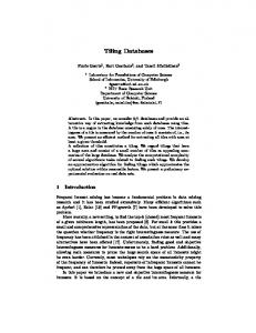
Figure 4.7: Tiling with 2-dimensional stencils. The thick arrows in (b) represent the dependence between tiles. Next step is to do subtile the parallelepiped tiles, by applying the same subtiling strategy in Figure 4.5-(a), so that the slope of the boundary planes between tiles is determined by the left projection of the dependence vectors on the < ⃗t,⃗i0 > and < ⃗t,⃗i1 > planes. As a result of this tiling strategy, four subtiles are generated: A,B0 , B1 and C, as shown in Figure 4.8-(a). The dependence relations among subtiles are: A → B0 , A → B1 , B0 → C, B1 → C and A → C. Subtile A and C are two pyramids of the same shape, but B0 and B1 are not pyramids. However, if w0′ = h + w0 /2 and w1′ = h + w1 /2, the projections of the subtiles on < ⃗t,⃗i0 > and < ⃗t,⃗i1 > planes are still conjugate trapezoids, as shown in Figure 4.8-(b). Figure 4.9-(a) shows the slice of a tile for one time step, where all the tiles are rectangles. Because of the dependences among subtiles, the computations in subtile A must be done first; then B0 and B1 (the order of B0 and B1 is not important because there are no dependences between them); and finally, C. Based on the dependences among tiles shown in Figure 4.7(b), each time step a tile only needs to send the data near the left and bottom boundaries (the shadowed area in the Figure) to the corresponding neighbor nodes. So only subtiles A, B0 and B1 send data, while subtile C, B0 and B1 receive data. There are five separate send operations: S0 (from A to the lower-left neighbor), S1 (from A to the left neighbor), S2 (from A to the neighbor below), S3 (from B0 to the neighbor below), and S4 (from B1 to the
59
w'0
w'1
C
B1 B0
t
i1 i0
A
(a) Subtiling
t A
t
B0
A
i0
B1
i1 (b) Projections of subtiles
Figure 4.8: Subtiling with 2-dimensional stencils. neighbor below). R0 , R1 , R2 , R3 and R4 are the corresponding receive operations. In total, each time step there are 14 computation and communication operations within a tile. Figure 4.9-(b) shows the order of these operations, as enforced by the dependences. Because each tile is assigned to a single node, we can schedule the above 14 operations in any sequential order that satisfies the dependencies in Figure 4.9-(b). In order to hide communication latency, it is necessary to delay the computation associated with receive operations. The start of the computation of subtile B0 and B1 can be delayed by h′ time steps from subtile A, so that the latency of transmitting the data from S1 and S2 to R1 and R2 , respectively, is hidden. However, in subtile C, the R3 and R4 need to receive the data from S3 and S4 in tiles, B0 and B1 , respectively. Hence execution of C should be delayed by h′ time steps from subtile B0 and B1 , or 2 × h′ time steps from subtile A. The projections of the subtiles after these delays are shown in Figure 4.10. The dashed trapezoids are the projections of the subtiles behind the others.
60
R3
R2
S4
B1
C
A
B0
R0 R4
S1
i1
S0
R1 S2
S3
i0 (a) Slice of a tile when t = t0 .
S1 (t0)
R1(t0-h')
B0
S4(t0-h')
R4(t0-2×h') R0(t0-2×h')
S0(t0)
A
R2(t0-h')
S2(t0)
stage 1
S3(t0-h')
B1
C
R3(t0-2×h')
stage 2 (delay h' )
stage 3 (delay 2×h' )
(b) Dependence among the operations within each time step.
Figure 4.9: Schedule of subtiles for each time step.∀j, Sj and Rj are the corresponding send and receive pair.
C
C
B1 t
B0 2×h'
B0 A
t A i1
h'
i0
2×h'
B1
h'
Figure 4.10: Projections of subtiles with 2-dimensional stencils.
4.2.4
Higher Dimensions
For ISLs with higher dimensional stencils, Conjugate-Trapezoid Tiling is more complicated. For example, the 3-dimensional Jacobi code is a 27-point stencil, where the iteration space is 4-dimensional and requires a 3 × 3 cube of elements to compute each output element.
61
Although we cannot draw the shape of 4-dimensional tiles, the approach discussed in Section 4.2.3 for a 3-dimensional iteration space can be used to apply tiling to the 4-dimensional iteration space. The 4-dimensional cone that contains all the dependence vectors is projected on to < ⃗t,⃗i0 >, < ⃗t,⃗i1 > and < ⃗t,⃗i2 > planes. Based on the projection of the dependence cone, we apply the same tiling strategy as in Figure 4.4 to produce parallelogram tiles on each 2-dimensional plane. The resulting tile is a 4-dimensional hyper-parallelepiped. Subtiles are computed as shown Figure 4.5-(a) on the projection of the hyper-parallelepiped tile on each plane, so that the projections of subtiles on each plane are conjugate trapezoids. The total number of subtiles within a tile is 23 = 8. For a given time step, the slice of a hyperparallelepiped tile is a cuboid, as shown in Figure 4.11, where subtile A send the boundary data to 7 neighbor nodes, and subtile D receive data from other 7 neighbor nodes. Thus, for each time step, the computation of subtile B0 , B1 and B2 depends on subtiles A, and subtiles C0 , C1 and C2 depend on subtiles B0 , B1 and B2 , and subtile D depend subtiles C0 , C1 and C2 . Hence, when delaying subtiles to hide communication latency, the subtiles are divided into four stages. The first stage includes subtile A, as well as the send and receive operations associated to A; the second stage, includes subtiles B0 , B1 and B2 , which are delayed by h′ time steps from subtile A; the third stage, includes subtiles C0 , C1 and C2 , that are delayed by 2 × h′ time steps; and the fourth stage includes the subtile D, which is delayed 3 × h′ time steps. C0 B2
D
C1 C2
B1
i2
i1 A i0
B0
Figure 4.11: Slice of a 4-dimensional hyper-parallelepiped tile. Based on the above discussion, the algorithm of Conjugate-Trapezoid Tiling for ISLs with 62
n-dimensional stencil ((n + 1)-dimensional iteration space) can be summarized as shown in Algorithm 1. Algorithm 1 Conjugate-Trapezoid Tiling for ISL with d-dimensional stencil ((d + 1)dimensional iteration space) ⃗ lef t (⃗t,⃗ij ) and B ⃗ right (⃗t,⃗ij ) of the cone of dependence vectors for each plane 1: Compute B < ⃗t,⃗ij > (j=0,1,...,d − 1). 2: Compute H = (⃗ hT0 , ⃗hT1 , ..., ⃗hTd−1 , ⃗hTd )T . Each row of H is the normal vector of a tiling hyperplane. The last row ⃗hd = (1/h, 0, 0, ..., 0). Other rows ⃗hj (j = 0, 1, ..., d − 1) are computed as follows: ( ) 1 ⃗ 0 1 ⃗ P roj (hj ) = · Bright (⃗t,⃗ij ) · −1 0 wj
3:
4:
5:
6:
The rest of the components in ⃗hj are filled with zeros. Tile the iteration space with the tiling hyperplanes defined by H. The height of each tile is h, and the width of each tile on ⃗ij dimension is wj . Distribute tiles on nodes organized in a d-dimensional mesh < ⃗i0 , ⃗i1 , ..., ⃗id−1 >. Divide the projection of the tile on each < ⃗t,⃗ij > plane into two conjugate trapezoid ⃗ lef t (⃗t,⃗ij ). This results in 2d subtiles. The boundary of between subtiles is parallel to B subtiles in each (d + 1)-dimensional tile in total. Partition the 2d subtiles into d + 1 stages according to the dependence among subtiles. Schedule the subtiles in order of stage. Delay the k-th stage by k × h′ time steps (k = 0, 1, .., d). In each subtile, receive necessary boundary data from neighbor nodes before computation, and send boundary data to neighbor nodes after computation.
4.3
Performance Model
This section introduces a performance model of Conjugate-Trapezoid Tiling which is used to the explain the experimental results.
63
4.3.1
Definitions
At each time step, the total number of stencil points computed by each node is:
Ncomp =
d−1 ∏
wj
j=0
Ncomp stands for the volume of the d-dimensional tile slice at each time step. The order of Ncomp is d. If the average computation time for each stencil point is tpoint , the computation time at each time step would be:
tcomp = tpoint · Ncomp = tpoint ·
d−1 ∏
wj
j=0
Only the data points at the boundaries of the tile need to be communicated (to be sent or received) with neighboring nodes. For 1-dimensional Jacobi, the total number of data points to be sent at each time step is 2. For 2-dimensional Jacobi, the grey area in Figure 4.9-(a) shows the data points to be sent. I assume that the messages sent to different destination nodes do not cause congestion with each other, so I only need to consider the largest message, which would cause the longest latency. The maximum number of data points to be sent at each time step is 2 · max{w0 , w1 }. In general, for a n-dimensional stencil, the maximum number of data points to be sent at each time step is:
Vsend = c · max{
n−2 ∏
wjk |∀⃗j = (j0 , j1 , ..., jn−2 )}
k=0
in which c is a constant determined by the stencil. For the Jacobi stencils of any dimension, c = 2, which means Jacobi stencil only requires each points to exchange data with its direct neighbor points. Intuitively, Vsend is proportional to the size of one ”surface” of the ndimensional tile slice at each time step, so the order of Vsend is n − 1. Because of symmetry,
64
for any non-boundary node, the volume of data to be sent is equal to the volume of data to be received, so let Vsend = Vrecv = V . For each send -receive pair, let tlatency denote the latency. In practice tlatency consists of two partss: the fixed startup overhead tstartup and the transmission latency which is determined by the size of the data to be transmitted:
tlatency = tstartup + ttrans · V For small messages, the total latency is dominated by the startup overhead, so tlatency ≈ tstartup . However, if the message is large, the total latency is proportional to the data size being transmitted: tlatency ≈ ttrans · V
∼
V
For each send or receive operation, even with asynchronous mode, there is some CPU time that cannot be overlapped with computations. Let tsend and trecv denote the overhead of asynchronous send and receive operations, respectively. Similarly, because of symmetry, for any non-boundary node the total number of send operations must be the same to the total number receive operations at each time step. Let Nsend = Nrecv = Nmsg . Nmsg is determined by the number of neighbor points that needs to do data exchange, which is a constant for a given stencil. Because the total number of neighbor points for a n-dimensional stencil is 3n − 1, the upper bound of Nmsg is (3n − 1)/2. For the Jacobi stencil, the values of Nmsg are 1, 3, 7 in the 1, 2, 3-dimensional cases, respectively.
65
4.3.2
Performance Model
If communication and computation are not overlapped, the total execution time at each time step is:
texec = tcomp + (tsend + trecv ) · Nmsg + tlatency = tpoint · Ncomp + (tsend + trecv ) · Nmsg +tstartup + ttrans · V
Consider the Conjugate-Trapezoid Tiling proposed in this paper. Let the total number ′ of points computed at each time step be Ncomp . At each time step in the steady state, ′ Ncomp ≈ Ncomp . Because of subtiling, the size of the message sent by each subtile is smaller,
so the maximum number of data points to be sent V ′ is smaller than V : V ′ ≤ V . The cost ′ ′ is that the total number of send or receive operations, Nmsg , becomes larger: Nmsg ≥ Nmsg . ′ For the Jacobi stencil, with subtiling the values of Nmsg are 1, 5, 19 in the 1, 2, 3-dimensional
cases respectively. The number of messages to be sent for 2-dimensional Jacobi. is shown in Figure 4.9-(a). Figure 4.12 shows the number of messages to be sent for 3-dimensional Jacobi. For standard tiling, 7 messages need to be send to different neighboring tile (1 message for the data on the vertex, 3 messages for 3 edges and another 3 for the 3 faces), as shown in Figure 4.12-(a). After Conjugate-Trapezoid Tiling, some messages are divided into 2 (the original edge messages) or 4 messages (the original face messages) due to subtiling, as shown in Figure 4.12-(b). However, those message that are divided from the same original message are still to be sent to the same destination tile. The total number of messages becomes 19. The increase of the number of the messages may cause performance problems, which will be addressed in Section 4.3.3. Because subtiles are delayed in Conjugate-Trapezoid Tiling, there are at least h′ time steps between each send and receive pair. Let t′exec denote the total execution time at each 66
′ (b) Nmsg = 19.
(a) Nmsg = 7.
Figure 4.12: Number of messages to be sent for 3-dimensional Jacobi. Each arrow stands for a message to be sent to an neighboring tile. The arrows with the same direction means that the destination of the messages are the same. time step with Conjugate-Trapezoid Tiling, and t′latency = tstartup + ttrans · V ′ is the latency of the largest message. Then if t′latency is smaller than the total execution time of h′ time steps, h′ × t′exec ≥ t′latency = tstartup + ttrans · V ′
the communication latency can be fully overlapped: ′ t′exec = t′comp + (tsend + trecv ) · Nmsg ′ ′ = tpoint · Ncomp + (tsend + trecv ) · Nmsg
(4.1)
According to above, the minimum number of delayed time step h′ to fully hide communication latency is determined by: t′latency tstartup + ttrans · V ′ = h ≥ ′ ′ ′ + (tsend + trecv ) · Nmsg texec tpoint · Ncomp ′
67
(4.2)
The performance benefit achieved by Conjugate-Trapezoid Tiling is: ∆ = texec − t′exec ′ = tpoint · (Ncomp − Ncomp ) ′ +(tsend + trecv ) · (Nmsg − Nmsg ) + tlatency ′ ≈ tlatency − (tsend + trecv ) · (Nmsg − Nmsg )
4.3.3
(4.3)
Optimization
Communication-Coalesce Optimization With Conjugate-Trapezoid Tiling, the number of send and receive operations at each time ′ step, Nmsg , is greater than Nmsg , which can cause performance degradation according to ′ Equation 4.3. Nmsg ≥ Nmsg is because the data to be exchanged with the same neighbor
node are divided into two or more messages by the delayed subtiles. For example, in Figure 4.9, the destination of message S1 and S4 is the same node. However, after schedule of subtiles, within the same time step t0 , S1 is provided by subtile A with the data stands for the original time step of t0 , but S4 is provided by subtile B0 with the data stands for the original time step of t0 − h′ . This leads to S1 and S4 becoming two separate sending operations, and so as S2 and S3 . If postpone S1 until the computation in subtile B0 completes, the send operations of S1 and S4 can be merged into one because the destination node is the same. S2 and S3 can also be merged by postponing S2 until subtile B1 is complete. Similarly, for receive operations if bring R4 forward before subtile B0 starts, R1 and R4 can be merged because they have the same source node, and so as R2 and R3 . Figure 4.13 shows how communication operations are merged. Compared to Figure 4.9-(b), S1 and S2 are postponed while R3 and R4 are moved into an earlier stage. This optimization of merging communication operations is always possible, because send opera68
S1 (t0)
R4(t0-2×h')
S1 (t0)
A
B0
R1(t0-h')
S4(t0-h')
R0(t0-2×h')
S0(t0) S2(t0)
R2(t0-h')
B1
S3(t0-h')
R3(t0-2×h')
stage 1
R4(t0-2×h')
C
R3(t0-2×h')
S2(t0)
stage 2 (delay h' )
stage 3 (delay 2×h' )
Figure 4.13: Merge communication operations. The send or receive operations with in the same dashed box can be merged. Compared to Figure 4.9-(b), the send or receive operations denoted by the dashed arrows are moved (delayed or brought forward) to the operations denoted by corresponding thick arrows. tions only need to be postponed, and receive operations only need to be moved to an earlier stage. This optimization still preserve the correctness of communication. Although S1 and R4 are the corresponding send and receive operations, and S1 and R4 are moved into the same stage as shown in Figure 4.13, there are still h′ time steps of execution between the corresponding send and receive operations in the pipeline (when S1 sends out the data for time step t0 , R4 is receiving the data for time step t0 − h′ ). Hence this optimization does not affect the threshold of h′ calculated in Equation 4.2. Because the send or receive operations with the same destination or source node are ′ merged into one operation, this optimization results in that Nmsg = Nmsg and V ′ ≈ V on
the steady state of the pipeline.
69
Balanced Multi-Threading If nodes have more than one processors, the computation can be evenly distributed to every processor because the stencil points at each time step are fully parallelizable. However, the overhead of asynchronous send or receive operations can not be reduced through parallelization. This optimization is to balance the overall load of computation and communication operations. As shown in Figure 4.14, the white bars stand for computation time, and the grey bars stand for communication operation overhead. When nodes work in sequential mode, ′ the total execution time of each time step is t′exec = t′comp + (tsend + trecv ) · Nmsg . If nodes work
in parallel mode, assume each node has 4 processors, the computations can be divided into partitions and distributed on to each processor. However, the overhead of communication operation cannot be divided. As a result, instead of evenly dividing the computations in into 4 partitions, the partition(s) which produces data for sending or depends on the data to be received are designed to contain less computations. So the overall load distribution is balanced. time t'exec Sequential Mode trecv ·N’op
t'comp
tsend ·N’op
Processor 0 Processor 1 Processor 2 Processor 3
Parallel Mode
t'exec /4
Figure 4.14: Balanced multi-threading with four processors. The white bars stand for computation time, and the grey bars stand for communication operation overhead. In general, if each node has P processors, and max{tsend , trecv } ≤ t′exec /P , ideally the execution time in parallel mode can be t′exec /P if work load among threads are well balanced. 70
This is equivalent to that the amortized overhead of each communication operation is also reduced by parallelization, even though that the communication operation it self is not parallelized.
4.4
Unified Tiling Representation
This section uses the unified tiling representation framework defined in Section 2.1 to describe the Conjugate-Trapezoid Tiling discussed in this Chapter. The application of Conjugate-Trapezoid Tiling focuses on regular ISLs with the format shown in Figure 4.2. For ISLs with n-dimensional stencils, the iteration space I is an (n + 1)dimensional hyper-cuboid, so the basis matrix of I is a diagonal matrix: T, 0, 0, ..., 0 0, N0 , 0, ..., 0 I = span(E) = span( 0, 0, N1 , ..., 0 ... 0, 0, 0, ..., Nn−1
).
The first dimension of I is the time dimension, consisting of the time steps of the ISL. The rest of the n dimensions are the space dimensions. The stencil of an ISL may contain m points, which means that the computation of each data points depends on m neighboring data points from the previous time step. This results in m dependence vectors d⃗0 , d⃗1 , ..., d⃗m−1 in the iteration space I. Because each time step only needs the results from the previous time step, the first component of each dependence
71
vector must be 1. So the dependence matrix D must have the following form: D=
1, ∗ 1, ∗ = . ... 1, ∗
d⃗0 d⃗1 ... d⃗m−1
Because the tile shape T is an (n+1)-dimensional parallelepiped, there must exist a tiling
matrix T :
⃗t0
⃗t1 T = , ... ⃗tn such that T = span(T ). Since the projection of T on < ⃗i0 ,⃗i1 , ...,⃗in−1 > is an n-dimensional hyper-rectangle, 1 to n rows of T must be:
⃗t1 = (w0 , 0, 0, ..., 0), ⃗t2 = (0, w1 , 0, ..., 0), ... ⃗tn = (0, 0, 0, ..., wn−1 ).
For the first row of T , ⃗t0 is determined by the height of the parallelepiped tile h and the dependence vectors. More specifically, the projections on ⃗t0 on each < ⃗t0 ,⃗ij > is parallel to ⃗ right (⃗t,⃗ij ): B ⃗ right (⃗t,⃗ij ). P roj (⃗t0 ) = cj · B
72
And because the height of the parallelepiped tile is h, the first component of P roj (⃗t0 ) must be h: ⃗ right (⃗t,⃗ij ) P roj (⃗t0 ) = (h, xj ) = cj · B According to above equations:
xj =
⃗ right (⃗t,⃗ij ) · (0, 1)T B · h, ⃗ right (⃗t,⃗ij ) · (1, 0)T B
j = 0, 1, ..., n − 1
⃗t0 = (h, x0 , x1 , ..., xj , ..., xn−1 ).
Since Conjugate-Trapezoid Tiling is tessellating tiling, the repetition matrix R = T . After tiling, there still exists ”horizontal” dependences (dependence vectors that are perpendicular to the dimension of ⃗t). The dependence matrix between tiles are as follows: ′ D =
1, ∗ 1, ∗ ... 1, ∗ 0, ∗ 0, ∗ ...
.
0, ∗ The rows in D′ with the first component 0 are the dependence vectors perpendicular to the ⃗t dimension. Because of these ”horizontal” dependences, not enough parallelism can be exposed among tiles if each tile are executed atomically (as shown in Figure 4.4). However, after subtiling and delaying dependent subtiles, tiles within the same level can be executed
73
in parallel. As a result, the following schedule of tiles become valid:
1 0 S = , ... 0 S(⃗i′ ) = ⃗i′ · S = (i′0 , i′1 , ..., i′n ) · S = i′0 .
Similar to overlapped tiling, the purpose of the technique of subtiling and delaying dependent subtiles is to make the above schedule S valid and expose enough parallelism for coarse grain tiles. To sum up, Table 4.1 shows the unified representation of Conjugate-Trapezoid Tiling.
4.5
Evaluation
In this section, Conjugate-Trapezoid Tiling is evaluated on a distributed memory machine and the experimental results are presented.
4.5.1
Target Platform
The measurement of the performance is done with a distributed memory cluster of 32 nodes. Each node has an Intel Xeon quad-core X3430 CPU at 2.4GHz. The nodes are interconnected with a gigabit Ethernet. The MPI environment is MPICH2. The compiler is GCC 4.7.2, with the option -O3.
74
1, ∗ 1, ∗ I, D = ... 1, ∗
Input
D′
T
1, ∗ 1, ∗ 1, ∗ ... 1, ∗ , after subtiling: D′ = 1, ∗ . ... 0, ∗ 1, ∗ 0, ∗ ... 0, ∗ h, x0 , x1 , ..., xj , ..., xn−1 ⃗t0 w0 , 0, 0, ..., 0 ⃗t1 = 0, w , 0, ..., 0 T = 1 ... ... ⃗tn 0, 0, 0, ..., wn−1
D′ =
xj = R S
⃗ right (⃗t,⃗ij )·(0,1)T B ⃗ right (⃗t,⃗ij )·(1,0)T B
· h,
j = 0, 1, ..., n − 1
R= T. 1 0 S= ... . 0
Table 4.1: Representation of Conjugate-Trapezoid Tiling
75
Stencil Input Dimension Size 1-D Jacobi 1 512K 2-D Jacobi 2 1024 x 512 3-D Jacobi 3 64 x 64 x 64 PathFinder 1 512K Poisson 2 1024 x 512 Biharmonic 2 1024 x 512 HotSpot 2 1024 x 512 Cell 3 64 x 64 x 64
Points of Stencil 3 9 27 3 5 13 9 27
Table 4.2: Benchmarks
4.5.2
Implementation
The Conjugate-Trapezoid tiling discussed in this chapter is implemented in the Cetus compiler [22], which is a source-to-source C compiler. The inputs to the compiler are the sequential C codes of the ISLs. The dependence analysis result of Cetus provides the stencils definitions of the ISLs, which is the input to the tiling algorithm. The implementation use the Omega library [23] to perform tiling operations on the iteration space polyhedron. The code generation of Cetus is modified to generate parallel code with MPI APIs. In order to implement the optimization discussed in Section 4.3.3, the computation within each node is parallelized with Pthreads instead of OpenMP.
4.5.3
Benchmark
The same 8 ISL programs are evaluated as benchmarks as in Chapter 3: 1,2,3-dimensional Jacobi, PathFinder, Poisson, Biharmonic, HotSpot and Cell. These benchmarks contains 5 different stencils, from 1-dimensional to 3 dimensional. The input size for each benchmarks is listed in Table 4.2. Table 4.3 shows different stencils and the corresponding dependence vectors.
76
Stencil
Dependence Vectors (1, −1), (1, 0), (1, 1) (1, 0, 0), (1, ±1, ±1), (1, 0, ±1), (1, ±1, 0) (1, 0, 0), (1, 0, ±1), (1, ±1, 0) (1, 0, 0), (1, ±1, ±1), (1, 0, ±1), (1, ±1, 0), (1, 0, ±2), (1, ±2, 0) ∀x = −1, 0, 1, ∀y = −1, 0, 1, ∀z = −1, 0, 1, (1, x, y, z)
Benchmark 1-D Jacobi, PathFinder 2-D Jacobi, HotSpot
Poisson
Biharmonic
3-D Jacobi, CELL
Table 4.3: Different stencils of the benchmarks
4.5.4
Experimental Result
Performance Overview Figure 4.15-(a) shows the speedup achieved by Conjugate-Trapezoid Tiling with different values of h′ . The baseline is the performance achieved by tiling with no communication overlap. On average, Conjugate-Trapezoid Tiling achieves 1.9X speedup when h′ = 4. Among all the benchmarks, the common trend is that, as the value of h′ becomes larger than 4, higher performance is achieved. If communication latency is longer than the computation time within a tile, increasing h′ will delay the dependent subtiles, which are the receivers of messages, so that larger portion of communication latency can be hidden. This trend exactly shows the motivation of Conjugate-Trapezoid Tiling. However, It can also be seen that after exceeding a certain threshold, there is very little or no performance gain by keeping increase h′ . This is because if h′ is already large enough to hide the entire latency, 77
Speedup Over No Overlap
3 No Overlap
2.5
h'=1 h'=2 h'=3 h'=4 h'=5 h'=6 h'=7 h'=8
2 1.5 1 0.5 0
1-D Stencils
3-D Stencils
2-D Stencils
(a) Speedup with the Communication-Coalesce optimization.
Speedup Over No Overlap
3 No Overlap
2.5
h'=1 h'=2 h'=3 h'=4 h'=5 h'=6
2 1.5 1 0.5 0
(b) Speedup without the Communication-Coalesce optimization.
Figure 4.15: Speedup with different values of h′ . The baseline is the performance achieved by tiling with no communication overlap. The figure shows the performance with h′ up to 6 for 2-dimensional stencils and h′ up to 4 for 3-dimensional stencils, because the trend shows that there would be no additional performance gains with a larger h′ .
78
there will be no extra benefit with an even larger h′ . Equation 4.2 in Section 4.3.2 discussed the threshold of h′ . In Figure 4.15, for the benchmarks with 1-dimensional stencils (1-D Jacobi and PathFinder), the threshold is 6 or 7, while for the benchmarks with 2-dimensional stencils (1-D Jacobi, Poisson, Biharmonic and HotSpot) the threshold is 3 or 4. What is more, for 3-D Jacobi and Cell, which are the benchmarks with 3-dimensional stencils, peak performance is achieved when h′ = 1. This can be explained by Equation 4.2 as follows. The input sizes for each benchmarks shown in Table 4.2 are chosen to make the number of stencil points allocated to each node be the same across all benchmarks. So Ncomp is the same each ′ ′ benchmarks, and so is Ncomp because Ncomp ≈ Ncomp . However the amount of computation
of higher dimensional stencils is usually larger than that of lower dimensional stencils, such as 1-D Jacobi (3 points) versus 2-D Jacobi (9 points). For higher dimensional stencils the amount of computation of each stencil point is larger, and more time consuming, too. This means that tpoint is larger for higher dimensional stencils, which contributes one factor that leads to a smaller threshold of h′ according to Equation 4.2. The other factor is that for ′ higher dimensional stencils each tile has more neighboring tiles, so Nmsg and Nmsg are also
larger. The above two factors makes a larger denominator in Equation 4.2, and a smaller threshold of h′ as a result.
Communication-Coalesce Optimization Figure 4.15-(b) shows the speedup achieved without the Communication-Coalesce optimiza′ tion introduced in Section 4.3.3. Since for 1-dimensional stencils Nmsg = Nmsg = 1, there
is no difference with or without the Communication-Coalesce optimization. So 1-D Jacobi and PathFinder are not included in Figure 4.15-(b). Compared to Figure 4.15-(a), it can be seen that 2-dimensional stencils benchmarks (2-D Jacobi, Poisson, Biharmonic and HotSpot) achieve a lower speedup without the Communication-Coalesce optimization. Another observation is that the peak performance is reached with a smaller h′ : without the 79
Cycles 100000
110000
180000
No Overlap
h'=1 h'=2 h'=3 h'=4 h'=5 h'=6 h'=7 h'=8
80000 60000 40000 20000 0 1-D Jacobi
2-D Jacobi
3-D Jacobi
CELL
Figure 4.16: Communication overhead with different h′ . optimization the peak performance is reached around h′ = 3 while in Figure 4.15-(a) the peak performance is reached around h′ = 4 for most 2-dimensional stencils benchmarks. ′ Because without the optimization, the additional overhead introduced by (Nmsg − Nmsg )
more send and receive operations, the execution time at each time step becomes longer. So fewer time steps are needed to overlap with communication latency. This problem is more serious for benchmarks with 3-dimensional stencils, since for those benchmarks, without the ′ optimization Nmsg = 19, which is much larger compared to Nmsg = 7. As shown in Figure
4.15-(b), 3-D Jacobi and CELL can only achieve very small speedup with any h′ . The overhead of additional communication operations almost kill the performance benefit gained by overlapping communication and computation.
Communication overhead Figure 4.16 shows the communication overhead with different h′ . The overhead is measured by the average number of cycles taken by each blocking receive call MPI_Recv. So this overhead shown in Figure 4.16 stands for the trecv plus the part of tlatency that is not overlapped with computation. The bar of ”No Overlap” corresponds to trecv + tlatency , which is the upper bound of the overhead shown in the figure. It can be seen that from 1-D Jacobi to 3-D Jacobi, as the dimension of the stencil increases, the value of trecv + tlatency also increases. This is because according to the performance model defined in Section 4.3.2, if assuming
80
that trecv and tstartup are constant, the other part of tlatency is proportional to the number of data points to be communicated (V , which is the volume of the data to be sent or received), and the order of V is d − 1. This means that because higher dimensional stencils have larger communication volume, the communication overhead, if not hidden by overlapping with computations, is higher. In Figure 4.16 the ”No Overlap” bar of CELL is lower than 3-D Jacobi. CELL and 3-D Jacobi share the same stencil, which means the number of data points to be communicated is the same. However, each data point of CELL only takes one byte storage, while each data point of 3-D Jacobi is a floating point value. So the actual communication volume V of CELL is smaller than that of 3-D Jacobi. As the value of h′ increases, the communication overhead decreases for every benchmark shown in Figure 4.16, because more portion of communication overhead is hidden by overlapping it with computations. This can explain the trend of performance shown in Figure 4.15. When h′ exceeds some threshold, communication overhead does not reduce any more because tlatency is fully hidden and the lower bound trecv is reached. As in Figure 4.15, benchmarks with higher dimensional stencils reach the lower bound sooner with a smaller h′ compared to benchmarks with lower dimensional stencils.
Input Size Sensitivity Figure 4.17 shows the speedup with different input size for 1-D and 2-D Jacobi. For both benchmarks, h′ reaches the threshold with a smaller value with larger input size. This is ′ because larger input size results in larger Nmsg and Nmsg . This makes the denominator in
Equation 4.2 larger and thus a smaller threshold of h′ . It also shows than for both benchmarks as the input size getting larger, the peak speedup achieved by Conjugate-Trapezoid Tiling is lower. This is because a larger input size leads to larger tile size if the total number of computation nodes remains the same. When the large tile size is large enough the program becomes CPU-bound instead of communication-bound. The optimization opportunity for 81
4
2.5
3 256K 512K 1024K 2048K
2.5 2 1.5 1 0.5 h'
0
Speedup Over No Overlap
Speedup Over No Overlap
3.5
2 768×384
1.5
1024×512 1440×720
1
2048×1024 0.5 h'
0
0 1 2 3 4 5 6 7 8
0
(a) 1-D Jacobi
1
2
3
4
5
6
(b) 2-D Jacobi
Figure 4.17: Input size sensitivity. hiding communication latency for a cpu-bound program is small.
4.6
Conclusion
This chapter discusses the design and implementation of a new tiling scheme called ConjugateTrapezoid Tiling for ISLs. The proposed tiling scheme divides each tile into subtiles, and schedules subtiles within each tile to overlap computation and communication. This chapter describes the tiling algorithm in polyhedron model, and compare Conjugate-Trapezoid Tiling and standard tiling analytically. The proposed tiling scheme is implemented in Cetus compiler to automatically generated code for d-dimensional stencils. Experimental results on a cluster show that Conjugate-Trapezoid Tiling is able to effectively reduce the overhead of communication latency, and achieves significant speedup over traditional tiling strategy.gy.
82
Chapter 5 Tile Shape Selection for Hierarchical Tiling In this chapter, the tile shape selection for hierarchical tiling is studied. In hierarchical tiling, tile shapes at different levels interact with each other and together determine execution time. This means that, in order to minimize execution time, simply selecting tile shape for each level separately will not necessarily lead to the optimal choice; optimal tile shape selection can only be achieved by tackling hierarchical tiling in a global manner. Figure 5.1 shows an example of different tile shape choices. Arrows represent the dependences between tiles. Dashed lines show the tiles that can be executed in parallel in a wavefront schedule. The numbers stand for the order of the execution the wavefronts. Suppose the iteration space of the loop nest has two dependences: d⃗0 = (1, 0) and d⃗1 = (0, 1). There are different possible tile shapes for each level of tiling. The most common choice is the square. In Figure 5.1(a), both levels use square tiles. The tiles along the same diagonal line can be executed in parallel. Assume that the computation time of each level 0 tile is one unit time, the total execution time of schedule of in Figure 5.1-(a) is 7×7 = 49 units of time. There are, however, better tile shapes. If the level 1 tile shape is changed to a parallelogram as shown Figure
83
Level 0 Tile Shape
(a)
Level 1 Tile Shape
Iteration Space
Execution time
7
7 6 5
6
7×7=49
5
1 2 3 4 1
2
3
4
11 (b)
4×11=44 10
4 3 2 1
9 1 2 3 4 5 67 8
11
(c)
10
7 1 6 2 3 5 4
7×11=77
9 1 2 3 4 5 67 8
Figure 5.1: Different tile shape choices for hierarchical tiling. Arrows are the dependences between tiles. Dashed lines represent the tiles that can be executed in parallel in a wavefront schedule. The numbers stand for the order of the wavefronts 5.1-(b), the total number of time unit of execution time becomes 4 × 11 = 44 < 49. However, parallelogram shaped tile is not always the best choice. If we also choose parallelogram tile for the level 0 tiling, as shown in Figure 5.1-(c), the total execution time would increase to 7 × 11 = 77 units of time (here it is assumed that the parallelogram tile at level 0 takes the same time to execute as the square tile.). A quantitative model can be used to find the optimal tile shape choice combination for each level of tiling to achieve minimal execution time.
84
5.1
Problem Definition
Given the iteration space I with the shape of n-dimensional hyper-parallelepiped, assume ⃗ek = (ek,0 , ek,1 , ..., ek,n−1 ), k = 0, 1, ..., n−1 are the n edge vectors of the hyper-parallelepiped, then the following matrix E is the basis matrix of I: ⃗ e 0 ⃗e1 E= . ... ⃗en−1
And I = span(E). Assume there are m dependences in I. The m dependence vectors d⃗0 , d⃗1 , ..., d⃗m−1 , forms an m × n dependence matrix D as follows: D=
d⃗0 d⃗1 ... d⃗m−1
.
Without loss of generality, I assume that m ≥ n and there are n dependence vectors that are linearly independent 1 . Then select a tile shape T with n-dimensional hyper-parallelepiped shape, and ⃗tk = (tk,0 , tk,1 , ..., tk,n−1 ), k = 0, 1, ..., n − 1 are the n edges of the hyper-parallelepiped tile, so the 1
Otherwise, it must be possible to make at least one loop full permutable through a sequence of affine transformations, and then it can be simplified into a lower dimensional iteration space.
85
following matrix T is the tiling matrix (the basis matrix of space T):
⃗t0
⃗t1 T = ... ⃗tn−1
.
As discussed in previous chapters, if using tile shape T(T) to tile the iteration space I, the tiled space I ′ is another n-dimensional iteration space. It is possible to apply tiling transformation for I ′ again. To describe an l-level hierarchical tiling, define a sequence of iteration spaces I0 , I1 ,..., Il : I1 = I ′
I0 = I,
and ∀k = 1, 2, ..., l, Ik is the tiled space of Ik−1 . This follows the bottom-up approach of hierarchical tiling. Since each Ik must have the shape of n-dimensional parallelepiped, define Ek is the basis matrix for Ik : ∀k = 0, 1, ..., l,
Ik = span(Ek ).
At each level of tiling, the tile shape is Tk . In order to simplify the problem, tile shapes are restricted to n-dimensional parallelepiped, too. Let Tk be the tiling matrix at each level, ∀k = 0, 1, ..., l − 1,
Tk = span(Tk ).
The tiles at different levels are scheduled independently. And each tile is executed atomically, which means there is no communication with other tiles at the same level before computation within it is completed. With the definitions above, the problem is how to select tile shapes T0 , T1 , ..., Tl−1 for 86
d0 t0
d2 d1 t1
Figure 5.2: Constraints of tile shape imposed by dependences. each level of tiling, so that with any valid scheduling of tiles on each level, the total execution time of the final loop nest is minimized.
5.2
Constraints on Tile Shape Selection
In the discussion of this chapter, tile shapes are restricted with hyper-parallelepiped. And the tiles on each tiling level are scheduled atomically. Besides, tiles are tessellating, which means there is no overlapped between tiles introduced to eliminate dependences. With the assumptions above, Figure 5.2 describes the constraints of tile shape selection imposed by dependences in general. In order to produce a valid tile shape, the infinite cone spanned by extending the tile edges ⃗t0 , ⃗t1 , ..., ⃗tn−1 must contain every dependence vector. For the example in Figure 5.2, ⃗t0 and ⃗t1 must not be in the shaded area. To describe the above observation formally, each dependence vector d⃗k must be covered by the cone spanned by the extension cords of ⃗t0 , ⃗t1 , ..., ⃗tn−1 , ∀d⃗k , ∃⃗a = (a0 , a1 , ..., an−1 ) ≥ ⃗0n = (0, 0, ..., 0)
(5.1)
d⃗k = a0 · ⃗t0 + a1 · ⃗t1 + ... + an−1 · ⃗tn−1 = ⃗a · T
Assume that every tile is always large enough so that inter-tile dependences only exist between adjacent tiles (including diagonal adjacent). This requirement can be expressed as
87
follows:
∀d⃗k , ∃⃗a = (a0 , a1 , ..., an−1 ) ≤ ⃗1n = (1, 1, ..., 1)
(5.2)
d⃗k = a0 · ⃗t0 + a1 · ⃗t1 + ... + an−1 · ⃗tn−1 = ⃗a · T
The above two requirements can be merged into the following:
∀d⃗k , ∃⃗a,
⃗0 ≤ ⃗a ≤ ⃗1,
d⃗k = ⃗a · T
(5.3)
which is the constraint imposed by dependences when choosing the tile shape. When the original iteration space I is tiled by matrix T and produces the tiled space I ′ , The relation among I, I ′ and T is studied as follows. First, assume the tiling transformation is an affine transformation, the shape of I ′ should still be an n-dimensional hyper-parallelepiped under any affine transformation. Suppose E ′ is the basis matrix of I ′ and I ′ = span(E ′ ), which is the space of tiles. There must be some n × n matrix A such that: E′ = E · A
Next, consider the effect of tiling transformation represented by A. As shown in Figure 2.4, after tiling, under the new coordinates system shown as axis labels i′0 and i′1 , vector ⃗t0 and ⃗t1 become (1, 0) and (0, 1), respectively. More generally, we have the following equation (1n denotes the n × n identity matrix):
⃗t0
⃗t1 T ·A= ... ⃗tn−1
1, 0, ..., 0 0, 1, ..., 0 ·A= ... 0, 0, ..., 1
88
= 1n
e0
(1,0)
dk=(2,2)
t0=(4,0)
(0,1) t1=(0,8)
e1 Figure 5.3: Inter-tile dependences (thicker arraows) generated by original dependence vector d⃗k . It can be concluded that A = T −1 . So the relation among I, I ′ and T is: E ′ = E · T −1 . So T −1 represents the affine transformation of the tiling transformation with tile shape T . When the original iteration space I is tiled by matrix T , each dependence vector d⃗k is also transformed to d⃗′ k by the affine transformation represented by T −1 . T must satisfy the constraints of Equation (5.3), d⃗′ k = d⃗k · T −1 = ⃗a · T · T −1 = ⃗a,
⃗0n ≤ ⃗a ≤ ⃗1n
(5.4)
As shown in Figure 5.3, a dependence vector (2, 2) would result in three dependence vectors after tiling: (1, 0), (0, 1), and (1, 1). In general, a single dependence vector d⃗k in original iteration space I generates one or more dependences between tiles in the tiled iteration space I ′ . The rule is that, for d⃗′ k = ⃗a = (a0 , a1 , ..., an−1 ), if aj > 0, there is a dependence (0, ..., 1, ..., 0) imposed on the j-th dimension in I ′ . In addition, if there are n dependence vectors d⃗k0 , d⃗k1 , ..., d⃗kn−1 which are linearly independent, the inter-tile dependences in I ′ generated by those n dependence vectors must include n orthonormal unit vectors. Considering the above observation in the context of hierarchical tiling defined in last section, if at the k-th level of tiling, the dependence matrix in iteration space Ik is Dk , Dk
89
must have the following form:
D0 = D, Dk =
d⃗k,0 d⃗k,1 ... d⃗k,m−1
1, 0, ..., 0
0, 1, ..., 0 1n = = , ... ∗ 0, 0, ..., 1 ...
∀d⃗k,j , k ≥ 1, 0 ≤ j < m,
5.3
⃗0 ≤ d⃗k,j ≤ ⃗1.
(5.5)
Execution Model
Assume that the sequential execution time only depends on amount of computation, and that the execution time of each iteration is always the same. So, if the computations of iteration space I = span(E) is not parallelized, the total execution time is proportional to the number of iterations within it:
T imes (I) = |I| = |det(E)|.
(5.6)
The execution time of a parallelized iteration space depends on the schedule of iterations within the iteration space. In order not to be tied to any specific scheduling scheme, the concept of ideal execution time is used in analysis. Ideal execution time is the minimal execution time of an iteration space I that can be achieved by any valid schedule of iterations. If each iteration in I is viewed as an activity and D represents the dependences between activities, the ideal execution time is determined by the critical path in I. It is assumed that there is infinite hardware parallelism available at each level. In practice, the above assumption means that the amount of hardware parallelism should be always larger than the 90
maximum number of iterations that can be executed in parallel. Under these assumptions, the critical path in I is the longest path of dependences between iterations. Let L(E, D) denote the length of the longest path of dependent iterations in the iteration space I with basis matrix E and dependence matrix D, the ideal execution time of I can be calculated as follows:
T ime(I) = L(E, D)
(5.7)
Section 5.4 discusses how to calculate L(E, D). In general, L(E, D) depends on every d⃗k in D. However, if the dependence vectors are not linearly independent, we can ignore some rows in D when calculating L(E, D). For example, the iteration space shown in Figure 5.4 has three dependence vectors d⃗0 , d⃗1 and d⃗2 , with d⃗2 = d⃗0 + d⃗1 . P and P ′ are two dependence paths within the iteration space. If there is any dependence path containing a pair of neighboring iterations with the dependence of d⃗2 , such as P ′ , it is always possible to replace d⃗2 on the path with a combination of d⃗0 and d⃗1 , as shown in Figure 5.4. This will resulting a longer dependence path. As a result, it can be concluded that the longest dependence path must only contain d⃗0 and d⃗1 (P ), and other dependence vectors can be ignored
2
when calculating L(E, D).
In particular, if there are n dependence vectors which are orthonormal unit vectors, it is safe to ignore other rows in D and only consider those n dependence vectors, because any other single dependence vector can be replaced by the combination of one or more orthonormal unit vectors, which will result in a longer dependence path. Based on above observation,
1n L(E, ) = L(E, 1n ) ∗ 2
Assume that the iteration space is much larger compared to each dependence vector.
91
(5.8)
݁Ԧ
ܲ ݀Ԧଶ
݀Ԧ
݀Ԧଶ
ܲ′ ݀Ԧ
݀Ԧଵ
݀Ԧଵ
݁Ԧଵ
Figure 5.4: The dependent pathes (P and P ′ ) within an iteration space. The length of a dependent path is the number of iterations on the path. If any path contains d⃗2 (P ′ ), it is always possible to replace d⃗2 with d⃗1 and d⃗0 on the same position, which resulting a longer path. This means the longest path (P ) must only contain d⃗0 and d⃗1 . According to Equation under the context of hierarchical tiling the dependence matrix 5.5, 1n each at each level Dk = , ∀k ≥ 1. As a result, Equation (5.8) can be used to simplify ∗ further analysis.
5.4
Calculate the Longest Dependent Path
When applying tiling transformations recursively to a given iteration space I, hierarchical tiling contains a tiling transformation at each level. Following a bottom-up approach for hierarchical tiling, first tiling matrix T0 is used to tile the original iteration space I0 = I, producing a new iteration space I1 . More generally, on the k-th level of tiling, tiling matrix Tk is applied to tile the iteration space Ik and generated the new iteration space Ik+1 . Assume Ek is the basis matrix of Ik ,
Ik = span(Ek ),
Ek+1 = Ek ·
Tk−1
= E0 ·
k ∏
Tj−1
j=0
The iterations in the bottom level tiles (the finest grain) are executed in sequential mode,
92
so the per-tile execution time can be calculated by Equation 5.6:
T ime(T0 ) = T imes (T0 ) = |det(T0 )| For upper level tiles (Tk , 1 ≤ k < l), each tile at the level immediately below is considered as a single iteration.Let Dk denote the dependences at the k-th level with D0 = D, the per-tile execution time is calculated using Equation 5.7:
T ime(Tk ) = L(Tk , Dk ) = T ime(Tk−1 ) · L(Tk , Dk )
Then the total execution time after tiling is:
T ime(I) = T ime(El ) = T ime(Tl−1 ) · L(El , Dl ) = T ime(Tl−2 ) · L(Tl−1 , Dl−1 ) · L(El , Dl ) = |det(T0 )| · (
l−1 ∏
k=1 l−1 ∏
= |det(T0 )| · (
L(Tk , Dk )) · L(El , Dl ) L(Tk , Dk )) · L(E0 ·
l−1 ∏
Tk−1 , Dl )
k=0
k=1
According to Equation 5.5 and 5.8, the above equation can be simplified to the following form: T ime(I) = |det(T0 )| · (
l−1 ∏
L(Tk , 1n )) · L(El , 1n )
(5.9)
k=1
So, the problem of optimal tile shape selection for hierarchical tiling is equivalent to selecting a sequence of tiling matrices T0 , T1 , ..., Tl−1 to minimize the above equation. Equation 5.9 does not include D; however, according to the discussion in Section 5.2 the shape of T0 must conform the constraints (Equation 5.1 and 5.2) imposed by each dependence vector in D.
93
5.4.1
Calculate L(Tk , 1n )
The meaning of L(Tk , 1n ) is the length of the longest dependent path with dependence matrix
1n in tile Tk . The iteration space in tile Tk can be normalized to an n-dimensional hyper cube by applying the affine transformation
3
represented by Tk−1 . Thus,
L(Tk , 1n ) = L(Tk · Tk−1 , 1n · Tk−1 ) = L(1n , Tk−1 ).
1n ⃗ Consider a row in 1n , d⃗j . Since Dk = , dj is also a row in Dk . Because Tk ∗ represents the tile shape at the k-th level of tiling, Tk must conform to the constraints imposed by each dependence vector in Dk . According to Equation 5.1 and 5.2: d⃗j = ⃗aj · Tk
∃⃗aj , ⃗0n ≤ ⃗aj ≤ ⃗1n ,
Then, let D′ denotes the dependences within the tile (normalized tile so that the tile is defined by tessellating edge vectors):
d⃗′ 0
d⃗′ 1 ′ D = ... d⃗′ n−1
d⃗0
⃗a 0 d⃗1 ⃗a1 −1 = 1n · Tk−1 = · Tk = ... ... ⃗ dn−1 ⃗an−1 ∀d⃗j ,
⃗0n ≤ d⃗′ j = ⃗aj ≤ ⃗1n
For the 2-dimensional cases, the intuitive explanation of the above observation is that the direction of each d⃗j must be in the upward, right or upper right direction, as shown in Figure In order to keep the problem in the integer domain, the affine transformation can be revised to Tk−1 · |det(Tk )|, and the discussion in this section would be still valid. 3
94
5.5 (a) and (b). Since the normalized iteration space is a hyper-cube, the longest path must start from the bottom left corner, which is the base point (0, 0, ..., 0). The problem of computing L(Tk , 1n ) is that finding the longest path P , which is a sequence of points p⃗0 , p⃗1 , ..., p⃗L−1 (Figure 5.5-(c), each p⃗1 stands for the coordinate of the point) such that:
p⃗0 = ⃗0 = (0, 0, ..., 0), ∀j = 0, 1, ..., L − 1, ⃗0 = (0, 0, ..., 0) ≤ p⃗j ≤ (1, 1, ..., 1) = ⃗1, ∃d⃗′ rj ,
p⃗j+1 = p⃗j + d⃗′ rj
(5.10)
L is the length of the dependent path found. Then L(Tk , 1n ) = max{L}. We have that the last point p⃗L−1 is defined as:
p⃗L−1
= p⃗L−2 + d⃗′ rL−2 =
L−2 ∑
d⃗′ rj
0 ≤ kj < n
j=0
= c0 · d⃗′ 0 + c1 · d⃗′ 1 + ... + cn−1 · d⃗′ n−1 = ⃗c · D′
⃗c = (c0 , c1 , ..., cn−1 ) ≥ ⃗0, ⃗c ∈ Zn
= ⃗c · Tk−1 Because ⃗0n ≤ d⃗′ j ≤ ⃗1n , the condition ⃗0 ≤ p⃗j ≤ ⃗1 is satisfied if ⃗0 ≤ p⃗L−1 ≤ ⃗1. And ∑ because n−1 j=0 cj is the total number of steps of the path, so max{L} can be solved through the following linear programming problem LP (Tk−1 , ⃗0, ⃗1): ⃗0 ≤ ⃗c · Tk−1 ≤ ⃗1,
⃗c ≥ ⃗0,
n−1 ∑ max{ cj }. j=0
Therefore, we conclude that L(Tk , 1n ) = LP (Tk−1 , ⃗0, ⃗1). 95
(5.11)
(1,0)
ݐԦ,
∙ ܶ
݀Ԧ
(1,0)
Ԧସ
ିଵ
Ԧଵ
�′�
݀Ԧଵ
Ԧଶ
Ԧଷ
�′�
ݐԦ,ଵ (a) Original tile
(0,1) (b) Normalized tile
Ԧ
(0,1)
(c) Dependent pathes
Figure 5.5: Determine the length of the longest dependent path within the iteration space of tile Tk . Each p⃗1 stands for the coordinate of the point.
5.4.2
Calculate L(El , 1n )
The meaning of L(El , 1n ) is the length of the longest dependent path in iteration space of the highest level tiling. Similarly, it is possible to apply the affine transformation represented by El−1 to normalize the iteration space: L(El , 1n ) = L(El · El−1 , 1n · El−1 ) = L(1n , El−1 ). Let D′ denote the transformed dependence matrix: D′ =
d⃗′ 0 d⃗′ 1 ... d⃗′ m−1
= 1n · El−1 = El−1
However, unlike the case when calculating L(Tk , 1n ), there is no guarantee that ∀d⃗′ j , ⃗0 ≤ d⃗j ≤ ⃗1. More intuitively, each dependence vector d⃗′ j can point to any direction. So L(El , 1n ) cannot be directly solved by the linear programming problem introduced in Equation (5.11). Since dependence vectors d⃗′ j can point to any direction, the longest dependent path does not necessarily start from base point (0, 0, ..., 0) of the hyper-cube iteration space. Thus the
96
dependent path P in the iteration space El is defined the same as in Equation 5.10 except that p⃗0 does not necessarily equal to ⃗0. To simplify the analysis, we define a related problem that is graphically depicted in Figure 5.6: find the longest path P ′ , which is a sequence of points p⃗′ 0 , p⃗′ 1 , ..., p⃗′ L′ −1 such that: p⃗′ 0 = (0, 0, ..., 0) = ⃗0, ⃗ = (−1, −1, ..., −1) ≤ p⃗′ L′ −1 ≤ (1, 1, ..., 1) = ⃗1, −1 ∀j = 0, 1, ..., L − 2,
∃d⃗′ rj ,
p⃗′ j+1 = p⃗′ j + d⃗′ rj
(5.12)
L′ is the length of path P ′ . P ′ starts from that base point, and only requires that the coordinate of the end point p⃗′ L′ −1 is within in the hype-cube surrounding the base point. p⃗′ L′ −1 can be calculated as follows: p⃗′ L′ −1 = p⃗′ L′ −2 + d⃗′ rL′ −2 =
L−2 ∑
d⃗′ rj
0 ≤ kj < n
j=0
= c0 · d⃗′ 0 + c1 · d⃗′ 1 + ... + cn−1 · d⃗′ n−1 = ⃗c · D′
⃗c = (c0 , c1 , ..., cn−1 ) ≥ ⃗0, ⃗c ∈ Zn
= ⃗c · El−1 ⃗ ⃗1): So max{L′ } can be solved through the following linear programming problem LP (El−1 , −1, ⃗ ≤ ⃗c · El−1 ≤ ⃗1, −1
⃗c ≥ ⃗0,
max{
n−1 ∑
cj }.
(5.13)
j=0
⃗ ⃗1) Next step is to prove that max{L′ } is approximately equal to max{L} so that LP (El−1 , −1, is a good approximation of L(El , 1n ). First, given any path P , it is always possible to construct a path P ′ by letting p⃗′ j = p⃗j − p⃗0 . So max{L} ≤ max{L′ } is easily proven. On the other hand, given a path P ′ , the start point is p⃗′ 0 = ⃗0, and the end point is 97
p⃗′ L′ −1 = (p′0 , p′1 , ..., p′n−1 ). In order to move path P ′ into the hyper-cubic space span(1n ), Construct ⃗s = (s0 , s1 , ..., sn−1 ) as follows: { ∀j = 0, 1, ..., n − 1
1,
pj < 0,
0,
else.
sj =
By shifting the offset of ⃗s, p⃗′ 0 and p⃗′ L′ −1 are moved into the hyper-cubic space span(1n ): ⃗0 ≤ p⃗′ s ≤ ⃗1,
p⃗′ s = p⃗′ 0 + ⃗s, p⃗′ e = p⃗′ L′ −1 + ⃗s,
⃗0 ≤ p⃗′ e ≤ ⃗1,
p⃗′ s ∈ span(1n ) p⃗′ e ∈ span(1n )
p⃗′ e = p⃗′ s + ⃗c · D′
(5.15)
Assume that the iteration space is much larger compared to the length of each dependence vector: ∀d⃗′ j , |d⃗′ j | L′ − ⌈
ε
⌉ = L′ − ε′ , ′ ⃗ min{|d j |} max{L} > max{L′ } − ε′ . The idea of above analysis is, we try to break path P ′ into small repeated pieces, and arrange the same number of repeated pieces in a line to construct P . Since the start and end points of P and P ′ are very close, the length of these two pathes should also be close. Figure 5.6 shows the intuition of above analysis. Since max{L} ≤ max{L′ } is already proved, it can be concluded that max{L} ≈ max{L′ }, with the error no larger than ε′ . As a result, the solution of the linear programming ⃗ ⃗1) can be used to estimate L(El , 1n ): problem LP (El−1 , −1, L(El , 1n ) = L(E0 ·
l−1 ∏
⃗ ⃗1) Tk−1 , 1n ) ≈ LP (El−1 , −1,
k=0
99
5.4.3
Summary
According to the discussion in last two sections, the problem of computing execution time of hierarchical tiled loop nests can be transformed into the following form:
T ime(I) = |det(T0 )| · (
l−1 ∏ k=1 l−1 ∏
≈ |det(T0 )| · (
L(Tk , 1n )) · L(El−1 , 1n ) ⃗ ⃗1) LP (Tk−1 , ⃗0, ⃗1)) · LP (El−1 , −1,
k=1
= f (E, T0 , T1 , ..., Tl−1 ) Given the basis matrix E of the original iteration space I, the optimal tile shape for hierarchical tiling is the sequence of tiling matrices T0 , T1 , ..., Tl−1 that minimize f (E, T0 , T1 , ..., Tl−1 ). If I is n-dimensional, each tiling matrix Tk contains n2 elements. In total function f has n2 · l variables. Besides, f is a non-linear function. Finally, because f contains terms of the solutions to linear programming problems, the problem of optimal tile shape selection is a multidimensional, nonlinear, bi-level programming problem.
5.5
Automatic Tile Shape Selection
According to the discussion in last section, optimal tile shape selection for hierarchical tiling is a multidimensional, nonlinear, bi-level programming problem, which is not easy to solve analytically. As a result, simulated annealing is adopted to select tile shape automatically according the analytical model introduced in last section. The sketch of simulated annealing algorithm to select tile shape is shown in Algorithm 2. Line 8 in Algorithm 2 valid(N ewS) checks whether the randomly generated N ewS is a valid tiling solution, otherwise N ewS will be generated again. This includes checking each Tk in N ewS satisfy the constraints imposed by dependences (Equation 5.1 and 5.2). This
100
Algorithm 2 Sketch of simulated annealing algorithm to select tile shape for hierarchical tiling ˚0 , T˚1 , ..., Tn−1 ˚ >; 1: Solution = Solution0 =< T ˚0 , T˚1 , ..., Tn−1 ˚ ); 2: T ime = f (E, Solution0 ) = f (E, T 3: Solutionbest = Solution; 4: T imebest = T ime; 5: Step = 0; 6: while Step < Stepmax do 7: N ewS = < T0 , T1 , ..., Tn−1 > =Solution + random(∆); 8: if valid(N ewS) then 9: N ewT = f (E, N ewS); 10: T emp = temperature(Step, Stepmax ); 11: if accept(N ewT, T ime, T emp, random()) then Solution = N ewS; 12: 13: T ime = N ewT ; end if 14: 15: if T ime < T imebest then 16: Solutionbest = Solution; 17: T imebest = T ime; 18: end if 19: Step = Step + 1; 20: end if 21: end while
101
also includes checking that the maximum number of parallelizable tiles does not exceed the hardware parallelism at each level. In addition, it is necessary to keep each tile large enough to aromatize the overhead of tiling. So we add an additional requirement in valid(N ewS) such that the iterations within each tile Tk much be more than a certain threshold T hk at each level of tiling: ∀Tk ,
|det(Tk )| ≥ T hk
Note that upper bound is not set for the size of each tile Tk . This is because the simulated annealing algorithm is self-adaptive and is able to converge to tiles with suitable size. The solution with very large tiles will lead to high execution time and hence the probability to be ˚ >, accepted in Line 11 of Algorithm 2 is low. For initial solution Solution0 =< T˚0 , T˚1 ,...,Tn−1 just choose the smallest possible tile that is valid for each level of tiling: |det(T˚k )| = T hk .
5.6
Unified Tiling Representation
The tiling schemes studied in this chapter are tessellating, atomic tiling, and the shape of iteration space and tile shapes are restricted to be n-dimensional hyper-parallelepipeds. As a result, there exists an basis matrix E such that I = span(E), and tiling matrix T such that T = span(T ). For tessellating tiling where the tile shapes are n-dimensional hyperparallelepipeds, the repetition matrix R = T . This chapter studies performance of the best possible schedule of tiles in stead of any particular scheduling scheme. Table 5.1 shows the unified representation of a single level of tiling. Because hierarchical tiling is done in the bottom-up approach in this chapter, the input for the kth level of tiling is: Ik = Ik−1 · Tk−1 , ′ Dk = Dk−1 .
102
Input
D′
T R S
I= span(E), D 1, 0, 0, ..., 0 0, 1, 0, ..., 0 0, 0, 1, ..., 0 ′ D = ... 0, 0, 0, ..., 1 ∗ the selected tile shape T R = T. Best possible S that minimizes the ideal execution time Table 5.1: The Unified Tiling Representation
5.7 5.7.1
Evaluation Environment Setup
Two platforms with hierarchical parallelism are step up for evaluation. One is the GPU platform consisting of an NVIDIA GeForce GTX 480 graphic card with 15 MPs and 480 SPs in total. The other platform is a 32-node cluster; each node has 4 Quad-Core AMD Opteron processors, or 16 cores. Because both platforms only have a 2-levels hierarchy, only 2-level hierarchical tiling is evaluated. For the GPU, the hardware parallelism at level 1 is 15, which is the number of MPs. However, although the number of SPs within each MP is 32, we consider the hardware parallelism at level 0 as 512 for the experiments. This is because NVIDIA GPUs require a certain number of concurrent hardware threads for each MP to achieve high throughput. For the cluster, the hardware parallelisms at two levels are 16 and 32, which are the number of cores per node and the total number of nodes. Two stencil computation programs are used as benchmarks: Gauss-Seidel and Jacobi. 1D stencils use 1-dimensional input array, and result in 2-dimensional iteration spaces, while 2-D stencils result in 3-dimensional iteration spaces. The iteration space of 1-D Gauss-Seidel contains two dependence vectors: (1, 0) and (0, 1), and the iteration space of 1-D Jacobi contains three dependence vectors: (1, −1), (1, 0) and (1, 1). There are three dependence 103
(1,0)
(1,-1)
(1,0)
(1,1)
(1,0,0) (0,1,0)
(0,1) (a) 1-D Gauss-Seidel
(0,0,1) (b) 1-D Jacobi
(c) 2-D Gauss-Seidel
Figure 5.7: The dependence vectors in the iteration space of stencil computation programs. vectors for 2-D Gauss-Seidel: (1, 0, 0), (0, 1, 0) and (0, 0, 1). Figure 5.7 shows the dependence vectors in the iteration space of stencil computation programs. An automatic system which uses simulated annealing is implemented to select tile shape for hierarchical tiling. The lp solve[8] is used to solve the linear programming problems in the model. The Omega Library[23] is used to do the tiling transformation and code generation. On the GPU platform, we generate OpenCL[24] code. On the cluster platform we generate hybrid MPI-OpenMP code: the higher level tiles are parallelized using MPI across nodes, and the lower level tiles are parallelized with OpenMP across processor cores within each node.
5.7.2
Performance
The performance of three common tiling schemes is compared with that of the code generated by our system: Wavefront, Diamond and Skewing, as shown in Table 5.2. The optimal sizes for the tiles of these three tiling schemes are chosen under the condition that the amount parallelism exposed does not exceed the hardware parallelism at the corresponding level. Figure 5.8 shows the speedup of the difference hierarchical tiling schemes for 2-dimensional the iteration spaces for both GPU and cluster platforms, and Figure 5.9 shows the performance data for 3-dimensional iteration spaces. The horizontal axis is the size of iteration space. The vertical axis is the speedup over Wavefront or Diamond. On average, the tiling 104
Wavefront
Tile Shape Tiling Matrix
(
x, 0 0, x
Diamond
)
(
x, −x x, x
)
Skewing
(
x, 0 −x, x
)
Table 5.2: Common tiling schemes: Wavefront, Diamond and Skewing. scheme with automatically selected tile shape can achieve over 90% speedup over Wavefront for Gauss-Seidel stencil, and 20%-30% speedup over Diamond for Jacobi stencil. The speedup achieved is consistent over different iteration space sizes. This means our automatic system can always find better tile shapes compared to common tiling schemes. For 1-D Jacobi stencil shown in Figure 5.8-(c) and (d), it can be seen that on the GPU platform Skewing shows a 10% speedup over Diamond, but no speedup is observed on the cluster platform. It is shown that the ideal execution times of Diamond and Skewing are the same for the Jacobi stencil. However, the amount of parallelism within each higher level tile varies less with Skewing than Diamond. This reason is that, as mentioned before, the execution model of NVIDIA GPU requires a certain number of concurrent hardware threads to achieve high throughput, Skewing shows better performance than Diamond on GPU.
5.7.3
Tile Shape
Table 5.3 shows the tile shape selection for 1-D Gauss-Seidel and Jacobi on GPU platform of each tiling scheme corresponding to Figure 5.8. Table 5.4 shows the tile shape selection for 2-D Gauss-Seidel on GPU. T0 and T1 are the tiling matrix at each level, and T0 ·T1 represents the tile shape in the original iteration space. In Table 5.3, under each matrix the shape of the tile is shown graphically. It can be seen that the common tiling schemes of Wavefront, Diamond and Skewing are combinations of regular tile shapes, including squares, diamonds
105
Wavefront ( ) 32, 0 0, 32
T0
( T1
( T1 · T0
256, 0 0, 256
8192, 0 0, 8192
Skewing ( ) 32, 0 0, 32
)
(
)
(
256, 0 −256, 256
Auto-Selected ( ) 2, −30 0, 12 )
8192, 0 −8192, 8192
(
)
(
256, −250 0, 56
512, −10680 0, 672
)
)
(a) 1-D Gauss-Seidel on GPU (128K×128K)
( T0
Diamond ) 18, −18 18, 18
( T1
( T1 · T0
256, 0 0, 256
(
)
4608, −4608 4608, 4608
(
)
(
Skewing ) 18, −18 18, 18
256, 0 −256, 256
4608, −4608 0, 9216
Auto-Selected ( ) −2, −18 8, 8
)
)
(
(
64, 0 −512, 512
)
−128, −1152 5120, 13312
)
(b) 1-D Jacobi on GPU (128K×128K)
Table 5.3: Tile shape selection for 1-D Gauss-Seidel and Jacobi.
106
Wavefront 2.5
Skewing
Auto-Selected
Wavefront 2.5
2
Auto-Selected
2 Speedup
Speedup
1.5 1
1.5 1
0.5
0.5
0
0
(a) 1-D Gauss-Seidel on GPU Skewing
(b) 1-D Gauss-Seidel on cluster
Auto-Selected
Speedup
Speedup
Diamond 1.4 1.2 1 0.8 0.6 0.4 0.2 0
Skewing
(c) 1-D Jacobi on GPU
Diamond 1.6 1.4 1.2 1 0.8 0.6 0.4 0.2 0
Skewing
Auto-Selected
(d) 1-D Jacobi on cluster
Figure 5.8: Hierarchical tiling performance for 2-dimensional iteration space on GPU and cluster platforms. The horizontal axis is the size of the iteration space. The vertical axis is the speedup over Wavefront or Diamond. and regular parallelograms. However, the automatically selected tile shapes are irregular parallelograms. Since it is nonintuitive to figure out the performance impact of a particular tiling scheme with irregular tile shapes (especially for higher dimensional iteration spaces), it is necessary to build an analytic model to evaluate tile shape selection quantitatively, and select tile shape automatically.
107
Wavefront
Wavefront
Auto-Selected
Auto-Selected
2.5 Speedup
Speedup
1.8 1.6 1.4 1.2 1 0.8 0.6 0.4 0.2 0
2 1.5 1 0.5 0
(a) 2-D Gauss-Seidel on GPU
(b) 2-D Gauss-Seidel on cluster
Figure 5.9: Hierarchical tiling performance for 3-dimensional iteration space on GPU and cluster platforms. The horizontal axis is the size of the iteration space. The vertical axis is the speedup over Wavefront. Wavefront 16, 0, 0 0, 16, 0 0, 0, 16 16, 0, 0 0, 16, 0 0, 0, 16 256, 0, 0 0, 256, 0 0, 0, 256
T0
T1
T1 · T0
Auto-Selected 16, −48, 0 0, 16, 0 0, −48, 16 8, −8, 0 0, 8, 0 0, −16, 16 128, −512, 0 0, 128, 0 0, −1024, 256
Table 5.4: Tile shape selection for 2-D Gauss-Seidel on GPU (1920×1920×1920).
5.7.4
Model Accuracy
Figure 5.10 compares the real execution time and the ideal execution time. The data is for 128K × 128K 1-D Gauss-Seidel running on GPU, with tile shape choices listed below:
32, 0 T0 = , 0, 32
256, 0 T1 = . x, 256
The value of x in T0 is scaled from 0 to −320. The shape of resulting T0 changes from a square to a parallelogram. It is shown that the trends of the real execution time and the 108
Real Execution Time (Milliseconds) Ideal Execution Time (Time Units) 3.5E+04
2.5E+07
3.0E+04
2.0E+07
2.0E+04
1.5E+07
1.5E+04
1.0E+07
1.0E+04
Time Units
Milliseconds
2.5E+04
5.0E+06
5.0E+03 0.0E+00
0.0E+00 0
-32 -64 -96 -128 -160 -192 -224 -256 -288 -320
Figure 5.10: Comparison between the real execution time and the ideal execution time for 1-D Gauss-Seidel. The left axis is for real execution time and the axis on the right is for ideal execution time. ideal execution time are exactly the same when tile shape varies. The result shows that ideal execution time commutated by the model in this paper can be used to direct tile shape selection.
5.8
Conclusion
In this chapter an analytical model is built to analyze the relation between the tile shape at each level of hierarchical tiling and the ideal execution time of the tiled loop nest. It is shown that the problem of optimal tile shape selection for hierarchical tiling is a multidimensional, nonlinear, bi-level programming problem. An automatic system which uses simulated annealing together with our analytical model is implemented to automatically select tile shape for hierarchical tiling. The tile shape selected by the automatic system can be quite different from the intuitive regular shapes. The experimental results show that irregular tile shapes may have the potential to achieve higher performance over regular tiling schemes. Currently the model focuses on the interaction between tile shape and parallelism exposure, and uses ideal execution time as the optimizing goal. The model could be more accurate by considering other factors affecting locality and communication. Besides, given 109
the complexity of the multi-dimensional nonlinear optimization problem in our model, at present simulated annealing is sued to find the near-optimal solution instead of the guaranteed optimal one. In future, it is possible to use the state-of-the-art optimization problem solving algorithms or libraries to solve the tile shape selection problem directly.
110
Chapter 6 Related Work Loop tiling is a traditional but effective optimization for programs whose execution time is dominated by loops, such as programs with stencil computations. Numerous optimizations based on the tiling of iteration spaces have been proposed for improving data locality [41, 44, 1, 2, 37, 14, 34, 40, 43, 47, 50], or exploiting parallelism [42, 45, 6, 19, 46, 7, 49]. Most of these works use polyhedral model as the representation of the tiling transformation. Bondhugula et al. design and implement Pluto [11], which can automatically transform loops for parallelism and locality based on the polyhedral model. Their transformation integrates traditional tiling techniques. However, existing research on tiling mainly focuses on tessellating tiling and scheduling tiles atomically. There have been ideas of taking advantage of the hierarchy of the hardware [30, 28, 33, 25, 10, 17, 9]. Hierarchical tiling as an effective optimization to exploit hardware hierarchy, has been proposed for better usage of memory hierarchy and enhancing parallel schedule [12, 18, 13]. For existing work on non-tessellating tiling, the closest work to the Overlapped Tiling discussed in this thesis is that of Krishnamoorthy et al.[27]. Their approach allows overlap between neighboring tiles to achieve balanced schedule of parallel tiles. Other works such as Ripeanu et al. [36] and Meng et al. [31] describe performance models to predict the
111
optimal amount of redundant computation for stencil computations in a grid environment with message passing or for GPUs, respectively. However, in those paper only single level of overlapped tiling is considered, so that as more communication/synchronization overhead is eliminated, the overhead introduced by redundant computations also increases in a higher order, which would kill the performance benefit of overlapped tiling. The most important difference between this thesis and existing work is the Hierarchical Overlapped Tiling transformation. Based on the observation that the overhead of redundant computation is the main drawback of the overlapped tiling approach, Hierarchical Overlapped Tiling applies overlapped tiling hierarchically. In this way, Hierarchical Overlapped Tiling is able to take advantage of the hierarchy of the hardware and provide more room of balance between the additional overhead introduced by redundant computation and the communication/synchronization overhead eliminated. The purpose of tiling with non-atomic tiles is usually to achieve balanced schedule when parallelizing tiles. When parallelizing ISLs, a typical strategy is to do loop skewing and wavefronting. However, wavefronting strategy would lead to an imbalanced schedule [27]. In order to achieve balanced schedule when tiling ISLs, Krishnamoorthy et al. [27] propose split tiling. The idea of split tiling is similar to Conjugate-Trapezoid Tiling: each tile is divided into sub-regions, and the sub-region without dependence is processed first, followed by the sub-regions with dependences. Since inter-tile communication needs to be done between the computation of sub-regions within a tile, split tiling is a tiling scheme with non-atomic tiles. On the other hand, split tiling can be also viewed as a tiling scheme with more than one tile shapes as discussed in Section 2.1.3, and the set of neighboring tiles with different shapes forms a hyper-parallelepiped-shaped super tile. Tang et al. [38] implement the Pochoir compiler, which automates a trapezoidal decomposition for stencil code. Their decomposition algorithm is very similar to split tiling. So it can be viewed as another example of tiling with non-atomic tiles. However, their work is based on shared memory machines, 112
and the inter-tile communication overhead is not studied. For split tiling and the Pochoir compiler, inter-tile communication is still aggregated at the beginning or end of the execution of tiles or subtiles/sub-regions; inter-tile communication is not interleaved with computations. So although the tiles/super-tiles are non-atomic, subtiles and sub-regions are still execution atomically. Because communication latency cannot be overlapped with computation time, the overall performance could still suffer from the overhead caused by communication latency. This might be tolerable for shared memory machines, but could cause performance problems for distributed machines, which is expected to have higher inter-node communication latency. Demmel et al. [15] proposed techniques to reduce communications for sparse matrix computations under distributed memory environment. Their technique allows communication during the execution within a tile, and schedule computation and communications to reduce the penalty of latency. However, their results show that speedups are only achieved for machines with very high communication latency; no speedup is achieved by their parallel algorithm on machines with fast network. On contrast, the Conjugate-Trapezoid Tiling introduced in this thesis can change the number delayed steps h′ to fit target platforms with different communication latency. It is well known that tile shape, as well as tile size, can have a significant impact on locality, inter-tile communication and parallelism [32, 48, 29]. However, most of the existing research on tiling mainly focus on choosing tile size assuming those of regular shapes (such as rectangles, or regular parallelograms) that can be produced with the help of simple auxiliary transformations such as loop skewing. This is because the performance impact of irregular tiles shapes is usually nonintuitive and it is not easy to develop a strategy to find a good tile shape among irregular shapes. Besides, it is also difficult to write code with irregular tiles manually. Xue [48] presents an approach to find the parallelogram or hyper-parallelepiped tile shape that is able to minimize the amount of communication between tiles. This work does not consider the impact of tile shape on parallel scheduling. H¨ogstedt et al. [19] intro113
duce a model to select the tile shape that minimizes the execution time. Since their work only consider a single level of tiling, their model shows that the complexity to determine of execution time when the tiles are parallelograms is equivalent to the complexity of linear programming problem. None of these works discussed above studies the tile shape selection problem in the context of hierarchical tiling. Renganarayana and Rajopadhye [35] have the closest work of using the model of linear programming problem to optimize tiling schemes. Their work presents a model to estimate the overall execution time of loop nests. Their framework determines the optimal tile sizes for hierarchical tiling by solving a convex optimization problem. However, their work only considers hyper-rectangle tiles, as well as the shape of the iteration space. Although it is more difficult to analyze the performance impact of hierarchical tiling with the general tile shapes, experimental results given in this thesis show that irregular tile shapes have the potential to achieve higher performance over regular shapes.
114
Chapter 7 Conclusions This thesis studies the application of tiling techniques for stencil compucations. previous studies of tiling optimizations mainly focused on a single level tiling, tessellating tiling, regular shape tile, and executing tiles atomically. This thesis discusses several novel tiling techniques, including hierarchical tiling, non-tessellating tiling, executing tiles non-atomically, irregular tile shapes, and combinations of these techniques. Contributions of this thesis include: • The introduction of a unified tiling representation framework to represent general tiling schemes, including non-tessellating tiling and executing tiles non-atomically. An automatic code generator is developed to facilitate this tiling representation framework, which was used for the evaluation of the proposed tiling schemes. • Overlapped Tiling and Hierarchical Overlapped Tiling are introduced in this thesis. They belong to the category of non-tessellating tiling. Both of these tiling schemes aim at eliminating communication/synchronization overhead by introducing redundant computation. The second scheme also takes advantage of hardware hierarchy to reduce the amount of redundant computation.
115
• The introduction of the design and evaluation of Conjugate-Trapezoid Tiling. ConjugateTrapezoid Tiling pipelines intra-tile computation and inter-tile communication, so that the communication latency can be hidden by overlapping with computation time. • A novel approach to the tile shape selection problem for hierarchical tiling. It is concluded that optimal tile shape selection for hierarchical tiling is a multidimensional, nonlinear, bi-level programming problem. Experimental results show that the irregular tile shapes have the potential to outperform intuitive tiling shapes.
116
Bibliography [1] W. Abu-Sufah, D. J. Kuck, and D. H. Lawrie. On the performance enhancement of paging systems through program analysis and transformations. IEEE Transactions on Computers, 30(5):341–356, May 1981. [2] N. Ahmed, N. Mateev, and K. Pingali. Tiling imperfectly-nested loop nests. In Proceedings of the 2000 ACM/IEEE conference on Supercomputing (CDROM), Supercomputing ’00, Washington, DC, USA, 2000. IEEE Computer Society. [3] M. Alpert. Not just Fun and Games. Scientific American, 4, 1999. [4] W. F. Ames. Numerical Methods for Partial Differential Equations. Academic, San Diego, CA, sencond edition, 1977. [5] C. Ancourt and F. Irigoin. Scanning polyhedra with DO loops. In Proceedings of the third ACM SIGPLAN symposium on Principles and practice of parallel programming, PPOPP ’91, pages 39–50, New York, NY, USA, 1991. ACM. [6] R. Andonov, S. Balev, S. Rajopadhye, and N. Yanev. Optimal semi-oblique tiling. In Proceedings of the thirteenth annual ACM symposium on Parallel algorithms and architectures, SPAA ’01, pages 153–162, New York, NY, USA, 2001. ACM. [7] R. Andonov and S. Rajopadhye. Optimal orthogonal tiling of 2-D iterations. Journal of Parallel and Distributed Computing, 45(2):159 – 165, 1997. 117
[8] M.
Berkelaar,
K.
Eikland,
and
P.
Notebaert.
Lpsolve.
http://lpsolve.sourceforge.net/5.5/. [9] G. Bikshandi. Parallel Programming with Hierarchically Tiled Arrays. PhD thesis, UIUC, 2007. [10] G. Bikshandi, J. Guo, D. Hoeflinger, G. Almasi, B. B. Fraguela, M. J. Garzar´an, D. Padua, and C. von Praun. Programming for parallelism and locality with hierarchically tiled arrays. In Proceedings of the eleventh ACM SIGPLAN symposium on Principles and practice of parallel programming, PPoPP ’06, pages 48–57, New York, NY, USA, 2006. ACM. [11] U. Bondhugula, A. Hartono, J. Ramanujam, and P. Sadayappan. A practical automatic polyhedral parallelizer and locality optimizer. In Proceedings of the 2008 ACM SIGPLAN conference on Programming language design and implementation, PLDI ’08, pages 101–113, New York, NY, USA, 2008. ACM. [12] L. Carter, J. Ferrante, and S. F. Hummel. Hierarchical tiling for improved superscalar performance. In Proceedings of the 9th International Symposium on Parallel Processing, IPPS ’95, pages 239–245, Washington, DC, USA, 1995. IEEE Computer Society. [13] L. Carter, J. Ferrante, S. F. Hummel, B. Alpern, and K.-S. Gatlin. Hierarchical tiling: A methodology for high performance. Technical report, 1996. [14] S. Coleman and K. S. McKinley. Tile size selection using cache organization and data layout. In Proceedings of the ACM SIGPLAN 1995 conference on Programming language design and implementation, PLDI ’95, pages 279–290, New York, NY, USA, 1995. ACM. [15] J. Demmel, M. Hoemmen, M. Mohiyuddin, and K. Yelick. Avoiding communication in sparse matrix computations. In Parallel and Distributed Processing, 2008. IPDPS 2008. IEEE International Symposium on, pages 1–12, April. 118
[16] Y. Duan, X. Zhou, W. Ahn, and J. Torrellas. Bulkcompactor: Optimized deterministic execution via conflict-aware commit of atomic blocks. In High Performance Computer Architecture (HPCA), 2012 IEEE 18th International Symposium on, pages 1–12, 2012. [17] B. B. Fraguela, J. Guo, G. Bikshandi, M. J. Garzar´an, G. Alm´asi, J. Moreira, and D. Padua. The hierarchically tiled arrays programming approach. In Proceedings of the 7th workshop on Workshop on languages, compilers, and run-time support for scalable systems, LCR ’04, pages 1–12, New York, NY, USA, 2004. ACM. [18] A. Hartono, M. M. Baskaran, C. Bastoul, A. Cohen, S. Krishnamoorthy, B. Norris, J. Ramanujam, and P. Sadayappan. Parametric multi-level tiling of imperfectly nested loops. In Proceedings of the 23rd international conference on Supercomputing, ICS ’09, pages 147–157, New York, NY, USA, 2009. ACM. [19] K. H¨ogstedt, L. Carter, and J. Ferrante. Selecting tile shape for minimal execution time. In Proceedings of the eleventh annual ACM symposium on Parallel algorithms and architectures, SPAA ’99, pages 201–211, New York, NY, USA, 1999. ACM. [20] W. Huang, M. R. Stan, K. Skadron, K. Sankaranarayanan, S. Ghosh, and S. Velusam. Compact thermal modeling for temperature-aware design. In Proceedings of the 41st annual Design Automation Conference, DAC ’04, pages 878–883, New York, NY, USA, 2004. ACM. [21] F. Irigoin and R. Triolet. Supernode partitioning. In Proceedings of the 15th ACM SIGPLAN-SIGACT symposium on Principles of programming languages, POPL ’88, pages 319–329, New York, NY, USA, 1988. ACM. [22] T. A. Johnson, S.-I. Lee, L. Fei, A. Basumallik, G. Upadhyaya, R. Eigenmann, and S. P. Midkiff. Experiences in using cetus for source-to-source transformations. In Proceedings
119
of the 17th international conference on Languages and Compilers for High Performance Computing, LCPC’04, pages 1–14, Berlin, Heidelberg, 2005. Springer-Verlag. [23] W. Kelly, V. Maslov, W. Pugh, E. Rosser, T. Shpeisman, and D. Wonnacott. The Omega Library interface guide. Technical report, 1995. [24] Khronos OpenCL Working Group. The OpenCL Specification, version 1.0.29, 8 December 2008. [25] I. Kodukula, K. Pingali, R. Cox, and D. Maydan. An experimental evaluation of tiling and shackling for memory hierarchy management. In Proceedings of the 13th international conference on Supercomputing, ICS ’99, pages 482–491, New York, NY, USA, 1999. ACM. [26] G. Kreisel and J.-L. Krivine. Elements of mathematical logic. North-Holland Pub. Co., 1967. [27] S. Krishnamoorthy, M. Baskaran, U. Bondhugula, J. Ramanujam, A. Rountev, and P. Sadayappan. Effective automatic parallelization of stencil computations. In Proceedings of the 2007 ACM SIGPLAN conference on Programming language design and implementation, PLDI ’07, pages 235–244, New York, NY, USA, 2007. ACM. [28] A. Leung, N. Vasilache, B. Meister, M. Baskaran, D. Wohlford, C. Bastoul, and R. Lethin. A mapping path for multi-gpgpu accelerated computers from a portable high level programming abstraction. In Proceedings of the 3rd Workshop on GeneralPurpose Computation on Graphics Processing Units, GPGPU ’10, pages 51–61, New York, NY, USA, 2010. ACM. [29] A. W. Lim, G. I. Cheong, and M. S. Lam. An affine partitioning algorithm to maximize parallelism and minimize communication. In Proceedings of the 13th international 120
conference on Supercomputing, ICS ’99, pages 228–237, New York, NY, USA, 1999. ACM. [30] J. Liu, Y. Zhang, W. Ding, and M. Kandemir. On-chip cache hierarchy-aware tile scheduling for multicore machines. In Proceedings of the 9th Annual IEEE/ACM International Symposium on Code Generation and Optimization, CGO ’11, pages 161–170, Washington, DC, USA, 2011. IEEE Computer Society. [31] J. Meng and K. Skadron. Performance modeling and automatic ghost zone optimization for iterative stencil loops on GPUs. In Proceedings of the 23rd international conference on Supercomputing, ICS ’09, pages 256–265, New York, NY, USA, 2009. ACM. [32] H. Ohta, Y. Saito, M. Kainaga, and H. Ono. Optimal tile size adjustment in compiling general DOACROSS loop nests. In Proceedings of the 9th international conference on Supercomputing, ICS ’95, pages 270–279, New York, NY, USA, 1995. ACM. [33] N. Park, B. Hong, and V. Prasanna. Tiling, block data layout, and memory hierarchy performance. IEEE Transactions on Parallel and Distributed Systems, 14(7):640–654, July. [34] J. Ramanujam and P. Sadayappan. Tiling multidimensional iteration spaces for nonshared memory machines. In Proceedings of the 1991 ACM/IEEE conference on Supercomputing, Supercomputing ’91, pages 111–120, New York, NY, USA, 1991. ACM. [35] L. Renganarayana and S. Rajopadhye. A geometric programming framework for optimal multi-level tiling. In Proceedings of the 2004 ACM/IEEE conference on Supercomputing, SC ’04, pages 18–, Washington, DC, USA, 2004. IEEE Computer Society. [36] M. Ripeanu, A. Iamnitchi, and I. T. Foster. Cactus application: Performance predictions in grid environments. In Proceedings of the 7th International Euro-Par Conference 121
Manchester on Parallel Processing, Euro-Par ’01, pages 807–816, London, UK, UK, 2001. Springer-Verlag. [37] Y. Song and Z. Li. New tiling techniques to improve cache temporal locality. In Proceedings of the ACM SIGPLAN 1999 conference on Programming language design and implementation, PLDI ’99, pages 215–228, New York, NY, USA, 1999. ACM. [38] Y. Tang, R. A. Chowdhury, B. C. Kuszmaul, C.-K. Luk, and C. E. Leiserson. The pochoir stencil compiler. In Proceedings of the 23rd ACM symposium on Parallelism in algorithms and architectures, SPAA ’11, pages 117–128, New York, NY, USA, 2011. ACM. [39] B. Virlet, X. Zhou, J. P. Giacalone, B. Kuhn, M. J. Garzaran, and D. Padua. Scheduling of stream-based real-time applications for heterogeneous systems. In Proceedings of the 2011 SIGPLAN/SIGBED Conference on Languages, Compilers and Tools for Embedded Systems, LCTES ’11, pages 1–10, New York, NY, USA, 2011. ACM. [40] M. Wolf, D. Maydan, and D.-K. Chen. Combining loop transformations considering caches and scheduling. International Journal of Parallel Programming, 26:479–503, 1998. [41] M. E. Wolf and M. S. Lam. A data locality optimizing algorithm. In Proceedings of the ACM SIGPLAN 1991 conference on Programming language design and implementation, PLDI ’91, pages 30–44, New York, NY, USA, 1991. ACM. [42] M. E. Wolf and M. S. Lam. A loop transformation theory and an algorithm to maximize parallelism. IEEE Transactions on Parallel and Distributed Systems, 2:452–471, October 1991. [43] W. Wolf and M. Kandemir. Memory system optimization of embedded software. Proceedings of the IEEE, 91(1):165–182, Jan. 122
[44] M. Wolfe. Iteration space tiling for memory hierarchies. In Proceedings of the Third SIAM Conference on Parallel Processing for Scientific Computing, pages 357–361, Philadelphia, PA, USA, 1989. Society for Industrial and Applied Mathematics. [45] M. Wolfe. More iteration space tiling. In Proceedings of the 1989 ACM/IEEE conference on Supercomputing, Supercomputing ’89, pages 655–664, New York, NY, USA, 1989. ACM. [46] D. Wonnacott. Time skewing for parallel computers. In Proceedings of the 12th International Workshop on Languages and Compilers for Parallel Computing, LCPC ’99, pages 477–480, London, UK, UK, 2000. Springer-Verlag. [47] D. Wonnacott. Achieving scalable locality with time skewing. International Journal of Parallel Programming, 30:181–221, 2002. [48] J. Xue. Communication-minimal tiling of uniform dependence loops. In Languages and Compilers for Parallel Computing, volume 1239, pages 330–349. Springer Berlin / Heidelberg, 1997. [49] J. Xue. Loop tiling for parallelism. Kluwer Academic Publishers, Norwell, MA, USA, 2000. [50] J. Xue and C.-H. Huang. Reuse-driven tiling for improving data locality. International Journal of Parallel Programming, 26:671–696, 1998. [51] X. Zhou, W. Chen, and W. Zheng. Cache sharing management for performance fairness in chip multiprocessors. In Parallel Architectures and Compilation Techniques, 2009. PACT ’09. 18th International Conference on, pages 384–393, 2009. [52] X. Zhou, J.-P. Giacalone, M. J. Garzar´an, R. H. Kuhn, Y. Ni, and D. Padua. Hierarchical overlapped tiling. In Proceedings of the Tenth International Symposium on Code 123
Generation and Optimization, CGO ’12, pages 207–218, New York, NY, USA, 2012. ACM.
124