TIME AGGREGATION OF NORMAL MIXTURE GARCH MODELS Carol Alexander and Emese Lazar ISMA Centre, School of Business, The University of Reading Whiteknights Park, PO Box 242 United Kingdom
[email protected] and
[email protected]
probabilities that any element of the population behaves according to each of the behavioral types ([9]).
ABSTRACT Normal mixture GARCH models capture the timevariation of variance, skewness and kurtosis that characterizes financial data. These models are more flexible and have been shown to offer a better fit than symmetric and asymmetric t-GARCH models. In this paper we give a weak definition for the normal mixture GARCH(1,1) model that is aggregating in time. This result paves the way for the analysis of the continuous time limits of such models.
Another feature of financial data that is widely accepted is the volatility clustering of returns. To capture this, the broad class of normal GARCH models was introduced by Engle (1982) and Bollerslev (1986) ([10] and [11]). They assume: yt = X t ' γ + ε t , ε t | I t −1 ~ N (0, σ t2 ) where It-1 represents the information set available at time t-1 and the conditional variance follows a deterministic process with autoregressive characteristics. The basic GARCH(1,1) conditional variance process for the errors is defined by:
KEY WORDS GARCH process, normal mixture, time aggregation
1. Introduction
σ t2 = ω + αε t2−1 + βσ t2−1 , ω > 0, α , β ≥ 0, α + β < 1
The empirical distributions of returns to financial assets are characterized by skewness and excess kurtosis ([1], [2], [3], [4] and [5]). One of the most flexible and tractable families of non-normal distributions that are able to capture the skewness and kurtosis commonly found in financial data is the normal mixture family ([6] and [7]).
The normal GARCH(1,1) process can account for some, but not all of the unconditional kurtosis in the data. Although the unconditional kurtosis can be greater under the t-GARCH process, where the conditional density of the errors is t-distributed ([12]) this model cannot account for the time variation in skewness and in kurtosis that characterizes the conditional distributions of financial asset returns ([13], [14], [15]) except if these are explicitly modeled as in [14], [16] and [17].
The normal mixture density function is given by: K
η ( x) = ∑ p iφ i ( x) i =1
K
∑ pi = 1
i =1
Many authors have considered simple normal mixture GARCH models, where the error term follows a normal mixture distribution ([18], [19], [20], [21], [22] and [23]). However most of these papers impose severe constraints on the dynamics of conditional skewness and kurtosis. Consequently Haas, Mittnik and Paolella (2004) introduced the general normal mixture NM(K)GARCH(p, q) process ([24]).
where [p1, p2,…, pK] is the positive mixing law and φ i ( x) = φ ( x; µ i , σ i2 ) are normal density functions. A random variable whose distribution is characterized by a density function of this form is denoted X ~ NM ( p1 ,..., p K ; µ1 ,..., µ K ; σ 12 ,..., σ K2 )
Alexander and Lazar (2005) provide an extensive analysis of the theoretical and empirical properties of the NM(K)GARCH(1,1) process and show that the general NM(2)GARCH(1,1) model offers a better fit than symmetric and asymmetric t-GARCH models ([25]). Moreover, time variation in conditional skewness and kurtosis is endogenous to the model.
Normal mixtures have a wide range of interpretations ([6], [4], [8]). From a behavioral point of view two major directions can be differentiated: (i) the mixing law determines the relative frequencies of the different behavioral types in the population and (ii) it gives the
437-033
210
The NM(K)-GARCH(1,1) process is defined in [25] by: (1)
Yt = X t' γ + ε t
(2)
σ t2 = ∑ p i σ it2 + ∑ p i µ i2 ,
K
K
i =1
i =1
K
∑ pi = 1
and
i =1
(3)
σ it2
= ω i + α i ε t2−1
+
β i σ it2−1
2. Time Aggregation Taking expectations in (2) shows that the total unconditional variance in the model can be expressed as a sum of two terms: the mean (under the discrete mixing law distribution) of the unconditional variances plus the variance (under the mixing law) of the conditional means of the components:
K
∑ pi µ i = 0
i =1
(5)
i = 1,…, K
(
2 ε t I t −1 ~ NM p1 ,..., p K ; µ1 ,..., µ K ; σ 12t ,..., σ Kt
K
( )
K
i =1
i =1
In this decomposition of the total variance we are interested in the relative contribution of each component variance, and to this end we define:
and according to the strong definition, the error term follows, conditionally, a normal mixture distribution: (4)
( )
E σ t2 = ∑ p i E σ it2 + ∑ p i µ i2
)
The application of this model should not be limited to econometric analysis. Since the commonly observed smile and/or skew in implied volatility surfaces results in excess kurtosis and/or skewness in the conditional densities of the underlying returns ([5]) neither the normal GARCH model, nor the t-GARCH model can be ‘smile consistent’. But since the NM(K)-GARCH(1,1) process (1) – (4) does capture time variation in the higher conditional moments, it is a more realistic candidate for GARCH option pricing.
( ) E (σ ) E σ it2
(6)
qi =
(7)
η it = q i ε t2 − σ it2
2 t
It is easy to see that E (η it ) = 0 . Re-writing (7) in the form
(
) (
η it = q i ε t2 − σ t2 + q i σ t2 − σ it2
)
we see that ηit captures two time-varying effects for each variance component: the deviation of the squared return from the overall conditional variance, and the difference between the conditional variance of the component and a proportion qi of the overall conditional variance.
To this end, the continuous-time limit of strong NM(K)GARCH models is derived in [26]. However, when the continuous-time limit of the model is under discussion, time aggregation of a time variant model naturally comes into question: is the model keeping its properties when analyzed under a different frequency?
In the following definition f can be any single-valued function. We also adopt the behavioral interpretation (ii) above, so that pi is the probability that the conditional variance process at time t is governed by the ith component variance. To formalize this notation we introduce a variable st ∈ [1, 2, …K] to denote the ‘state of nature’ at time t.
Obviously, the assumption (4) does not guarantee time aggregation: a simple counter example is that the sum of two NM(K) distributed variables will, in general, be NM(2K) distributed and not NM(K). So already shifting from a time-step of length m to a step of length 2m we loose time aggregation. Also, a special technique is needed to take care of the dependence of the conditional variance on all previous disturbances. Exactly the same problem arises even in the simple normal GARCH(1,1) process. This problem has been studied extensively by Drost and Nijman ([27]) who subsequently defined a ‘weak’ normal GARCH(1,1) process that is invariant under changing the length of the time interval of observations. Their result has no straightforward generalization to the normal mixture GARCH(1,1) process.
Definition A random variable Yt is said to follow a weak NM(K)GARCH(1,1) process if, in addition to (1), (2), (3), (6) and (7) the following properties hold:
The purpose of this short paper is to derive a definition that is weaker than (4) under which the time aggregation property for normal mixture GARCH(1,1) processes does hold. This definition can later be used to study the continuous-time limit of the model.
211
(8)
P(st = i) = pi
(9)
E (ε t | s t = i ) = µ i ,
(10)
E (ε t f (ε t −1 , K , ε 0 )) = 0 ,
(11)
Corr η it , η it − j = 0 ,
(12)
Corr η it , ε u ε u − j = 0 ,
(
(
)
)
j>0 j>0
Note that the weak NM(K)-GARCH(1,1) process is not an exact generalization of the strong NM(K)GARCH(1,1) process. It can be shown that under (4) some, but not all the correlations defined in (11) and (12) are exactly zero. However, those that are not zero are extremely small (less than 0.01 and 0.0005 respectively) and we believe they tend to zero as the sample size tends to infinity, although this has yet to be proved.
Example (m=2): 2ωi
α
2 + β i − 2 β i q i
2 α i = qi
In the following theorem the variance process for the ith component, based on time-steps of length m is defined by:
i
and 2 β i ∈ (0,1) is the solution to: 2 βi
2 2 2 m σ i ,tm = m ω i + m α i ⋅ m ε (t −1) m + m β i ⋅ m σ i ,(t −1) m
(13)
α = ω i 1 + i + β i qi
1+ 2 β i2
for i = 1,…, K.
=−
− ce + d
(1 + c )e + f , 2
where: Theorem The class of weak NM(K)-GARCH(1,1) processes is closed under temporal aggregation. After annualization, the parameters of m σ it2 are given by:
α c = i + β i qi d=
m
α 1 − i + β i qi mωi = ωi αi + β i 1 − qi
e=
m βi
βi
1+ m β i2
α i q + β i i
( ) E (η )
4q i2 E ε t2 ε t2−1 2 t
2
2
Proof of Theorem: From (3) we have: α σ it2 = ω i + i + β i q i ε t2−1 − β iη it −1 qi
= −Corr (v it , v it − m )
This can be rearranged as:
where v it =
α α − β i i + β i − β i 1 + i q qi i
2
∈ (0,1) is the solution to m
qi
α α α α f = 1+ 1+ i + i − βi i + βi + βi i + βi qi qi qi qi
m α i + β − β = α q m i i i m i q i
and
αi
2
2
α α qi ε t2 = ω i 1 + i + β i + i + β i qi ε t2−2 + q q i i α α + η it + i η it −1 − β i i + β i η it −2 qi qi
1 2 m −1 min ( p ,m ) ∑ ∑ c k η i ,t − p + 2 p =0 k =max (0, p +1− m )
m α + ∑ ε t −r ε t − s − i + β i ε ε ∑ t − m − r t − m − s 0≤ r < s < m q 0 ≤ r < s < m i
Repeating this equation for t – 1 and summing yields: 2
α α q i ⋅ 2 ε t2 = ω i 1 + i + β i + i + β i q i ⋅ 2 ε t2− 2 qi qi
and 1 k −1 α α c k = i i + β i qi qi m −1 αi − β i β + i q i
2
α + q i ε t ε t −1 − q i i + β i ε t − 2 ε t −3 q i
if k = 0
αi αi η + 1 + α i η η it − 2 + − + β β 1 it it − i i q q q i 1 i i + 2 αi + β i η it −3 − β i q i
if 1 ≤ k ≤ m − 1 if k = m
212
Obviously E (wit ) = 0 . Also, it can be shown that:2
where we have used the following relationship for annualized returns: 2 2εt
(14)
Corr (wit , wit − 2 k ) = 0 for k ≥ 1.
= (ε t + ε t −1 )2 / 2 = ε t2 / 2 + ε t2−1 / 2 + ε t ε t −1
Rewriting (17) as
Letting
v it = wit − λi wit − 2
(18) 2
vit = q i ε t ε t −1
α − q i i + β i ε t − 2 ε t −3 qi
we have: α q i ⋅ 2 ε t2 = ω i 1 + i + β i q i
αi α η + 1 + α i η − β i i + β i η it − 2 it it −1 + qi 1 qi qi + 2 αi + β i η it −3 − β i qi
2
α + i + β i q i ⋅ 2 ε t2− 2 + wit − λi wit − 2 qi
that is:
we can now write 2
α α q i ⋅ 2 ε t2 = ω i 1 + i + β i + i + β i q i ⋅ 2 ε t2− 2 + vit qi qi
(19)
and it is easy to see that:
E (vit vit − 2 k ) = 0 Corr (v it , vit − 2 ) =
(20)
for k > 1
x 1+ x
2
e + ec 2 + f
(21)
2 2σ t
= ∑ p i ⋅ 2 σ it2 + ∑ p i µ i2
K
K
i =1
i =1
and this is the updating formula for the new two-period conditional variances of each component. Equations (10) 2
Let c 2 k = Corr ( wit , wit − 2 k ) . From (16) and (18) we
(
We now define wit in the following way:
)( (
))
have that c 4 = c 2 1 + λi4 / λi 1 + λi2 . Assuming c 2 ≥ 0 (the case for c 2 ≤ 0 follows similarly) we have c 4 ≥ c 2 . Applying (15) similarly we obtain that c 2( k +1) ≥ c 2 k , with equality only if c 2 = c 4 = K = 0 .
wi 0 = vi 0 and wit = v it + λi wit − 2
Summing (15) for k = 2, 3,… gives
1
First, it can be shown that a is negative. Also: 1 − < a Ù e + ec 2 + f > 2ce − 2d which is true because 2 1 + c 2 > 2c and f + 2d > 0 , being a sum of squares.
(
= q i ⋅ 2 ε t2 − wit .
2 α i + β − λ q ⋅ ε 2 + λ ⋅ σ 2 i i i 2 it − 2 q i 2 t −2 i
= −a .
λi − Corr (vit , vit − 2 ) = 1 + λi2
(17)
2 2 σ it
Hence (19) becomes: αi 2 2 σ it = ω i 1 + q + β i + i
Hence there exists 0 < λi < 1 such that: (16)
)
Also, let:
−ce + d
Denoting the above correlation by a, we have a ∈ (1/2, 0).1 Consider the function f ( x) = x 2 + a −1 x + 1 for a ∈ (1/2, 0). Since f is continuous, f (0) = 1 and f (1) < 0, f must have a root x between 0 and 1. And if f ( x) = 0 , then
(
Now, similarly to (7), we define
E (vit ) = 0
(15)
α qi ⋅2 ε t2 − wit = ωi 1+ i + β i + qi 2 α i + β − λ q ⋅ ε 2 + λ q ⋅ ε 2 − w i i it −2 i 2 t −2 i i 2 t −2 q i
∞
(1 − λi )2 ∑ c 2k k =2
+ λi (c 4 − c 2 ) = 0
which holds only if c 2 k = 0 for k ≥ 1.
)
213
and (11) for the new two-step NM(K)-GARCH(1,1) model (replacing η by w and using steps of length 2) are obviously satisfied. Equation (12) can also be proved easily using the results derived above. The proof for mperiod time intervals follows by induction. QED
4.5
3.5
Corollary: The transformation of the parameters within the time aggregation keeps the unconditional (individual and overall) annualized variances constant.
2.5
Proof of Corollary: Taking expectations in (14) gives:
1.5
(22)
1
( ) ( )
E 2 ε t2 = E ε t2
4
16
64
256
1024
Fig. 1. The excess kurtosis of the DJ index implied by the NM(2)-GARCH(1,1) model as function of the step length
Equations (7) and (20) result in: (23)
( )
( )
(
)
( )
E σ it2 = q i E ε t2 and E 2 σ it2 = q i E 2 ε t2
3. Conclusion
Combining (2), (20), (21) and (22) will lead to:
Hence the unconditional overall and individual variances remain unchanged as the time interval changes.
NM(K)-GARCH(1,1) models are gaining popularity due to their ability to capture time-varying higher moments. Still, as with simple normal GARCH(1,1) models, the usual ‘strong’ definition has the deficiency that when different time steps are considered, the number of normals in the normal mixture distribution changes.
Note that the Theorem holds irrespective of the new mstep values for p i and µ i . In theory these could change in any way we like. For instance, we could introduce a simple parameterization for these parameters so that they change systematically over time. Naturally, we would require their definition to preserve the stylized properties of moments in accordance with the central limit theorem.
This paper has introduced a weak definition for NM(K)GARCH(1,1) models that is time aggregating, i.e. when discrete-time returns are measured at different time intervals, the model remains a valid description of the data using any step length. We obtained that the unconditional variance is not affected by the step length, but the kurtosis decreases as longer steps are considered.
Suppose we define
Consequently, it is legitimate to study the continuous-time limit of this model using the weak definition. The advantage of using diffusion limits of discrete-time models is that they offer more advanced tools for option pricing and hedging than the discrete-time model on its own.
(
) ( )
E 2 σ t2 = E σ t2
(23)
m
p i = p i and
m µi
= µi
for annualized returns. Then the unconditional skewness, which only depends on the unconditional variances and the parameters p and µ, will be unaffected by the time step change. However, we still have a term structure for kurtosis, even under the simple assumptions (23).
An empirical study testing the accuracy of the formulae derived is desirable. More than this, the study of the continuous-time limit of weak NM(K)-GARCH(1,1) models is of major interest (work in progress) and the main test will be to see how well these continuous models perform for option pricing and hedging.
The analytical relationship between the kurtosis’s computed using different time steps is fairly complex, but we have found that the kurtosis is a convex, generally decreasing function of the step length. To illustrate this, we estimated a NM(2)-GARCH(1,1) model for the Dow Jones index for the period of 2 Jan 1980 – 7 Sep 2004. Based on the estimated parameters and using the updating formulae given above we computed kurtosis values for different time steps (see Fig. 1). The excess kurtosis decreases when returns are measured at longer time steps, in accordance with the central limit theorem. 214
[15] D.B. Nelson, Asymptotic filtering theory for multivariate ARCH models, Journal of Econometrics, 71, 1996, 1-47
References: [1] B. Mandelbrot, The variation of certain speculative prices, Journal of Business, 36, 1963, 394-419
[16] C.R. Harvey, & A. Siddique, Autoregressive conditional skewness, Journal of Financial and Quantitative Studies, 34(4), 1999, 465-487
[2] E. Fama, The behavior of stock-market prices, Journal of Business, 38, 1965, 34-105 [3] J.M. Westerfield, An examination of foreign exchange risk under fixed and floating rate regimes, Journal of International Economics, 7, 1977, 181-200
[17] C. Brooks, S.P. Burke & G. Persand, Autoregressive conditional kurtosis, ISMA Centre Discussion Papers in Finance Series 2002-5, 2002
[4] J.W. McFarland, R.R. Pettit, & S.K. Sung, The distribution of foreign exchange price changes: Trading day effects and risk measurement, The Journal of Finance, 37(3), 1977, 693-715
[18] M.C. Roberts, Commodities, options, and volatility: Modelling agricultural futures prices, Working Paper, The Ohio State University, 2001
[5] G. Bakshi,, N. Kapadia, & D. Madan, Stock return characteristics, skew laws, and the differential pricing for individual equity options, The Review of Financial Studies, 16(1), 2003, 101-143
[19] P.J.G. Vlaar, & F.C. Palm, The message in weekly exchange rates in the European monetary system: Mean reversion, conditional heteroscedasaticity, and jumps, Journal of Business & Economic Statistics, 11(3), 1993, 351-60
[6] C.A. Ball, & W.N. Torous, A simplified jump process for common stock returns, Journal of Financial and Quantitative Analysis, 18 (1), 1983, 53-65
[20] L. Bauwens, C.S. Bos, & H.K. van Dijk, Adaptive polar sampling with an application to a Bayes measure of Value-at-Risk, Tinbergen Institute Discussion Paper TI 99-082/4, 1999
[7] S.J. Kon, Models of stock returns – A comparison, The Journal of Finance, 39(1), 1984, 147-165
[21] X. Bai, J.R. Russell, & G.C. Tiao, Beyond Merton’s utopia (I): Effects of non-normality and dependence on the precision of variance using high-frequency financial data, University of Chicago, GSB Working Paper July, 2001
[8] T.W. Epps, & M.L. Epps, The stochastic dependence of security price changes and transaction volumes: Implications for the mixture-of-distributions hypothesis, Econometrica, 44(2), 1976, 305-321
[22] X. Bai, J.R. Russell, & G.C. Tiao, Kurtosis of GARCH and stochastic volatility models with non-normal innovations, Journal of Econometrics, 114(2), 2003, 349360
[9] F. Mercurio, A multi-stage uncertain volatility model, Banca IMI Working Paper, 2002 [10] R.F. Engle, Autoregressive conditional heteroscedasticity with estimates of the variance of United Kingdom inflation, Econometrica, 50(4), 1982, 987-1007
[23] Z. Ding, & C.W.J. Granger, Modeling volatility persistence of speculative returns: A new approach, Journal of Econometrics, 73, 1996, 185-215
[11] T. Bollerslev, Generalized autoregressive conditional heteroskedasticity, Journal of Econometrics, 31, 1986, 309-328
[24] M. Haas, S. Mittnik, S. & M.S. Paolella, Mixed normal conditional heteroskedasticity, Journal of Financial Econometrics, 2(2), 2004, 211-250
[12] T. Bollerslev, A conditionally heteroskedastic time series model for speculative prices and rates of return, Review of Economics and Statistics, 69, 1987, 542-547
[25] C. Alexander & E. Lazar, Normal mixture GARCH(1,1). Applications to exchange rate modeling, Journal of Applied Econometrics, forthcoming
[13] D.S. Bates, The crash of ’87: Was it expected? The evidence from options markets, Journal of Finance, 46, 1991, 1009-1044
[26] C. Alexander & E. Lazar, The Continuous Limit of Normal Mixture GARCH, ISMA Centre Discussion Papers in Finance 2004-10, 2004
[14] B.E. Hansen, Autoregressive conditional density estimation, International Economic Review, 35, 1994, 705-730
[27] F.C. Drost & T.E. Nijman, Temporal aggregation of Garch processes, Econometrica, 61(4), 1993, 909-927
215