Time-bounded Localization Algorithm based on Distributed Multidimensional Scaling for Wireless Sensor Networks Ferdews Tlili
Abderrezak Rachedi
Abderrahim Benslimane
French University of Egypt University of Paris-Est (UPEM) ENSI, University of Manouba Informatics Research Center (CRI) Computer Science lab. (LIGM UMR8049) HANA Research Group Cairo, Egypt Marne-la-Vallee, France Tunis, Tunisia Email:
[email protected] Email:
[email protected] Email:
[email protected]
Abstract—Many applications of Wireless Sensor Networks (WSN) require to achieve the positions of the sensor nodes within a given time bound. In this paper we study the relative and physical localizability of WSN in a given time bound. We propose a new distributed and time bounded localization algorithm based on Multidimensional Scaling (MDS) method in WSN called D-MDS localization time algorithm. We compare the proposed algorithm to the existing algorithm based on the wellknown Trilateration method. The simulation results show that the proposed algorithm outperforms the existing approach based on Trilateration method in terms of the number of localized nodes in the network and the number of anchors required to physically localize the sensors. The D-MDS localization time algorithm localizes a large number of nodes for a low node degree in a time bound. Moreover it is able to physically localize the network with a low number of anchors compared with the algorithm based on Trilateration method. Index Terms—Wireless Sensor Networks, Localization algorithm, Localizability, Multidimensional Scaling (MDS), Local Coordinate System.
I. I NTRODUCTION Wireless Sensors Networks (WSN) are composed of many sensing-nodes that collect and gather information about the environment. For years, many researches have been focused on different limitations of WSN such as the connection of WSNs to the Internet [1], the management of the distributed data base for WSN [2] and the localization of nodes in WSNs [3]. In this work, we tackle the problem of localization in wireless sensors networks. The position information of sensor nodes has an important role for many applications of Wireless Sensor Networks (WSN). The sensor nodes require knowing their positions in order to track the objects [4] and to route the packets by using the geometrical routing [5]. The issue of localization is widely dealt with in order to improve localization accuracy where many techniques [3] and technologies [6] are used. However, many military and civilian systems require to confine the localization time. In literature, the localization time is a recent topic. In [7], Cheng et al. describe a study of the time bounded localization for WSN. They define a localization time algorithm based
on multilateration method. The main objective of relative and physical localization time algorithm is to maximize the number of localized nodes in a given time bound and to minimize the number of anchors required to physically localize the network. In this paper, we propose to use Multidimensional Scaling (MDS) method as a basic method for localization time algorithm. The aim of MDS [8] applied to localization is to find a map of sensor nodes positions, such that the distances between nodes fit as well as possible a given set of measured pairwise dissimilarities (e.g., distance between sensors measured using Received Signal Strength (RSSI)). The MDS method is easy to apply for the localization of sensors compared with Trilateration method. Indeed, for MDS method, the node requires a single measure of distance to any neighbor node to calculate its relative position. However, for Trilateration method, the node requires the distances to at least three localized and non collinear nodes in order to compute its position. Moreover the MDS method outperforms Trilateration method in terms of position accuracy as shown in [9]. That’s why, in this work we propose a new distributed and time bounded localization algorithm based on the MDS method. In addition, we evaluate the performance of the proposed algorithm, and we compare it with Cheng et al. algorithm [7]. The remainder of this paper is organized as follows: In section II, we propose a look over the related works. Then, we present a preliminaries for time localization in section III. We describe the localization time bounded algorithm based on the MDS method in section IV. In section V, we analyze the time complexity of our proposed algorithm. The simulation results are discussed in section VI. Finally, the conclusion and future work are given in section VII. II. R ELATED WORK In literature, there are various distributed localization algorithms [10]. These algorithms can be classified into two categories: full distributed iterative localization algorithms [11] [12] and cluster-based localization algorithms [13] [14].
The full distributed iterative localization algorithms [11] [12] consist in calculating the positions of unlocalized nodes which have at least the distance with three non collinear localized nodes at each iteration. The sensor nodes with known location information (or with the local coordinate system (LCS)) are called anchors. The new localized nodes are considered as anchors which contribute to localize other nodes in the next iteration. The main problem of this category of algorithms is that the localization errors propagate from one iteration to another. In the cluster-based localization algorithms [13] [14], each node and its one hop neighbors are localized in a local coordinate system (LCS). Thereafter, the clusters having three common and non collinear nodes are merged in a single cluster. The propagation of localization error in the network is reduced thanks to these algorithms. However, as the clusterbased localization algorithms are based on self localization of sensor nodes using the distance assessments, the error of distance assessments can influence the unique localizability of the network. This phenomenon is known as ”Flip ambiguity” in rigid graph theory [15]. Flip ambiguity is the reflection of a vertex position caused by a set of neighbors. In fact, a sensor node might have two different positions with the same distance assessment. In [15] and [16], the authors proved that the global rigidity of graph is a sufficient condition for unique localizability of the network. In this paper, we tackle the problem of localization time for the cluster-based localization algorithms. In [7], Cheng et al. carry out the first study of time bounded localization. They propose a distributed algorithm for time bounded localization based on Trilateration method. This approach consists of calculating the local positions of nodes in a local coordinate system. Then the local coordinate systems are merged together into a global coordinate system. The main limitations of this algorithm are the low number of localized nodes in the network for the small node degree and the large number of anchors required to physically localize the network. In this work, we aim to deal with these problems. We propose as a solution a distributed algorithm based on Multidimensional Scaling (MDS). We focus on the classic metric MDS [17]. The word classic is related to a single matrix of disparity used, and the word metric because the information of disparity is quantitative (measure of distances). The sensor positions using the classic metric MDS approach are calculated by decomposing into eigenvalues the double centered squared distance matrix. The distance matrix is composed of all distance assessments between each pair of nodes. The distances between nodes are calculated by using the received signal strength (RSS) measurements. III. P RELIMINARIES A. System Model We modeled a Wireless Sensor Network (WSN) as a graph G (V, E), where each vertex v ∈ V represents a sensor node, and each edge e ∈ E connects two vertices that are in communication range of each other. The graph is undirected
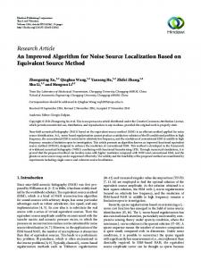
with edges weighted by the distance assessments. We choose to model the network as weighted graph for the reason that our proposed algorithm require that each node has the knowledge about its neighborhood especially which are its neighbors and the distances between the node and its neighbors. This model simplifies the application of our proposed algorithm. Figure 1 shows an example of graph model with five nodes connected by seven edges.
Fig. 1.
An example of network modeled by a graph.
B. The distributed MDS method Usually the MDS method is employed as a centralized approach for the network localization. Nevertheless, the distributed variant of MDS method is more appropriate to support the scalability of localization systems. In the distributed variant of MDS method [18] [19], individual nodes compute their own positions and the positions of their neighbors by using their local information in a Local Coordinate System (LCS). LCS is a relative coordinate system to the node. Each node calculates its position and the positions of its one hop neighbors using the metric MDS method. Thereafter the local coordinate systems are merged to form a Global Coordinate System (GCS) by using the linear transformation [20]. The linear transformation is to translate the coordinates of nodes from one coordinate system to another. This rotation between two coordinate systems is ensured by using at least three common and non collinear nodes in 2 − D space (or four in 3 − D space). C. Localizability of the network at a given time bound In this subsection, we explain the relative and absolute localizability of network at a given time bound [7]. Initially, we give some definitions: • Round of communications: it represents the granularity of time to assess the network localization time. One round of communications refers to the time required by the localized sensors to transmit their positions and to receive the positions of localized neighbors. • LCS Island (LCSI): is a set of mutually convertible local coordinate systems. For any two LCSs from different islands are not convertible to each other when the WSN has a disconnected graph topology [7]. • Time Localization: is the number of communication rounds required to merge all the LCS of each island in a single LCS.
•
•
•
Time Essential Localization: is the number of communication rounds expected to translate each LCS to any LCS island [7]. The relative localizability of network at a given time bound: a wireless sensor network is relatively localizable in k rounds of communications if and only if all sensor nodes are localized in their local coordinate systems and all local coordinate systems converge to only one LCSI in k communication rounds. The physical localizability of network at a given time bound: the necessary and sufficient condition for the physical localizability of network with n anchors in k rounds of communications consist in terminating the localization process within k rounds of communications and finding a location configuration of n anchors to convert the relative positions of nodes to absolute ones. In fact, for any isolated island, it requires at least three anchors for 2D localization (four anchors for 3D localization) in order to convert the relative coordinates of sensors to the absolute ones.
Fig. 2.
Fig. 3.
First case of the estimation of distance.
Second case of the estimation of distance.
IV. R ELATIVE AND A BSOLUTE L OCALIZATION T IME OF W IRELESS S ENSOR N ETWORK In this section, we describe the proposed distributed timebound localization algorithm based on MDS called D-MDS. We begin this section by explaining the assessments of the distance between sensor nodes. A. Distance Estimation First, each sensor node calculates the distances to its neighbors by using the Received Signal Strength (RSS) measurements. Thereafter, each node computes its distance matrix after exchanging its distance table with its neighbors. The distance matrix contains the distances between the node and its neighbors and the distances between each two neighbors. When two sensors are not within the communication range of each other they cannot calculate the distance between them by using the RSS assessments. The missing distance between two neighbors can be estimated (as illustrate in Figures 2 and 3). In Figure 2, the sensor node Np is placed in the middle of its neighbors N1 and N2 . The circles in the figure represent the communication range of the nodes. The distance between N1 and N2 can be estimated as follows: d ≈ d1 + d2
(1)
In Figure 3, the neighbors N1 and N2 are placed in the same side of the node Np . The distance between N1 and N2 can be approximated by this value: d ≈ |d1 − d2 |
d1 + d2 + |d1 − d2 | 2
Mode of operation of D-MDS Localization Time Algorithm.
(2)
Usually the distance between two neighbors is estimated by the average of distance of the previous two cases: d≈
Fig. 4.
(3)
B. Algorithm Process Figure 4 illustrates the flowchart of the proposed distributed time-bound localization algorithm called D-MDS. The first step of D-MDS consists in defining the local position of each node and its neighbors. After computing the distance matrix,
each node calculates its local position and the positions of onehop neighbors using the MDS method. The nodes initialize the following data structures: • • •
A position table, it contains the positions of the node and its neighbors in their local coordinate system. An identification table, it stores the identification of sensor that belong to the LCS. A transformation table, it specifies the transformation between each LCS in the identification table and a Base LCS (BLCS). The BLCS is an LCS that contains the maximum number of localized nodes.
The BLCS is selected as follows: After collecting the position tables of all neighbors at each communication round and based on the number of localized nodes in each LCS, each sensor chooses its BLCS that is the LCS which localizes the maximum number of nodes. The second step consists in merging each LCS to any isolated LCS island. After collecting the position tables, each node updates its identification table and selects its BLCS. Once the BLCS is selected, two steps are performed to update the transformation table: 1) a sensor checks its position table to find all the LCSs that can be transformed to the BLCS; 2) the sensor converts all LCSs identified in the first step into the selected BLCS. Finally, the sensor node updates its position table. Based on the results of D-MDS algorithm, we can study the localizability of network at a given time limit. In the one side, if iteration ≤ k where k is the limit of localization time defined by user and the number of LCS Island = 1 and the number of unlocalized nodes = 0, the sensor network is k-round relative localizable. In the other side, the physical localizability of network can be studied in terms of number of anchors required to physically localize the network. In fact, a sensor is k − round physical localizable if iteration ≤ k and the number of anchors required is defined as follows: number of anchors = 3 × number of Islands + number of unlocalized nodes
(4)
V. C OMPLEXITY A NALYSIS In this section, we analyze the complexity of time-bounded localization algorithm based on MDS method. In this proposed algorithm, each sensor node computes simultaneously its position and the positions of its neighbors in a local coordinate system (LCS) using MDS method. As MDS method consists of eigenvalue decomposition of the distance matrix, the time complexity is O(β 3 ), where β is the maximum node degree. The time complexity of computing n local coordinate systems is O(nβ 3 ), where n is the number of nodes in the network. We note that the time complexity of computing all the local coordinate systems is polynomial to the number of nodes in the network. Therefore, the D-MDS scheme is suitable for the large scale sensor networks.
A. Time complexity of time-bounded relative localization The local coordinate systems (LCS) are merged together to form the LCS islands (LCSI). The coordinates of two LCS are converted to each other if and only if there exist at least three (or four) nodes that are aware of their positions in both LCS in the two dimensional space (or in three dimensional space). The transformation of all LCSs into the LCSIs takes at most O(nL2 ) time, where n is the number of nodes and L is the number of possible LCS in the network. The number of possible LCS in the network is O(n) because initially each node constructs its LCS. When the network is not relative localizable in k communication rounds the network will be composed of many LCSI. Lemma 5.1: A network that is k-hop and d + 1-edgeconnected graph is relatively localizable in the k rounds of communications for the d-dimensional space. Proof: On the one hand, each two LCSs can be transformed to each other thanks to the d+1-edge connectivity of the graph. In fact, there exists at least d + 1 common nodes between each two LCSs. Therefore, all LCSs can be merged in only one LCS Island. On the other hand, as the network is k-hop graph, the LCSs converge to the unique LCS Island in at most k rounds of communications. According to the definition in section III-C, the k-hop and d + 1-connected network is k relatively localizable network. Moreover, the time complexity of checking the relative localizability of network in k rounds of communications is S = O(n × L × α) × O(nL2 ), where α is the diameter of network. Note that the time complexity is polynomial to the number of nodes in the network. As given in [7], the complexity of relative localization based on Trilateration method is O(n2 ) × O(nH 2 ), where n is the number of nodes in the network and H = O(n × β d ) is the number of possible LCSs for Trilateration algorithm in d-dimensional space. We note that our proposed algorithm outperforms the localization time algorithm based on Trilateration method in term of the time complexity. In fact, the D-MDS algorithm is faster to check the relative localizability of the network at a given time bound. B. Time complexity of time-bounded physical localization A linear transformation is applied to transform the relative positions into the absolute positions. Given sufficient number of anchors, the time complexity of computing the absolute positions of sensor nodes is O(a3 + n), where a is the number of anchors and n is the number of nodes in the network. The total time complexity of physical localizing the network is T = O(nβ 3 ) × O(nL2 ) × O(a3 + n). The main question to answer is the minimum number of anchors expected to physically localize the network at a given time bound. First, the isolated nodes that can’t be localized in any LCSI are chosen as anchors. Then, the theorem in [7] specifies the minimum number of anchors expected to physically localize the network. In fact, for a given network with diameter α, the lower bound of the number of anchors to physical localize the network in k communication rounds
is the ]}, where rootpositive is NA = max{3, [rootpositive min min 3 0 minimum positive root of the equation CN = H and A 2 α H 0 = k2 is the minimum number of LCSI required to cover the network [7]. VI. P ERFORMANCE E VALUATION In this section, we analyze the performances of the distributed time-bound localization algorithm D-MDS. We implement D-MDS by using MATLAB simulator. Then, we evaluate the proposed algorithm by comparing it to the time-bound localization algorithm based on Trilateration method [7].
B. Simulation results We evaluate the performances of our proposed algorithm in terms of the number of unlocalized nodes, the number of localized nodes in the largest Island, the percentage of localized nodes, the number of Islands, the number of anchors to physically localize the network and the time of localization which is quantified by the number of communication rounds. Then, the obtained results are compared with existing timebound localization algorithm based on Trilateration [7].
A. Simulation parameters The system is composed of 100 nodes randomly deployed in a two-dimensional squared area with size 100m × 100m. We vary the transmission range of nodes from R1 = 10m to R2 = 20m in order to range the average node degree approximately from 3 to 13. In each simulation, all the nodes have the same communication range. We change randomly the topology of the network 580 times in order to have over 50 network instances for the most node degrees. A network instance is a topology of network for a specific node degree. Table I defines all simulation parameters and their values. Parameter Number of nodes Lower bound of transmission range Upper bound of transmission range Deployment area Number of network instances
Value 100 10m 20m 100m × 100m 580
TABLE I T HE PARAMETERS OF SIMULATION AND THEIR VALUES
As the transmission range of nodes varies randomly, the degrees of nodes cannot be directly controlled. Therefore, Figure 5 shows the number of instances for each node degree that appears in the simulations. All simulation results afterward are the average of the results of all instances for each node degree.
Fig. 5.
The number of network instances for each node degree.
Fig. 6.
Variation of unlocalized nodes versus degree of nodes.
In Figure 6 , both curves are decreasing when the node degree increases. This is due to the fact that when the node degree raises the number of the nodes which satisfy the conditions of localization also increases for both algorithms. Moreover, it is apparent from the Figure 6 that the number of unlocalized nodes of our proposed algorithm is less than five nodes for the average node degree 3, while the number of unlocalized nodes of the Trilateration based algorithm is more than 25 nodes for the same average node degree. The reason of this large gap of the unlocalized nodes number between the two algorithms is that the nodes which have a degree equal to one or two are localized by the proposed algorithm; however these nodes are not localized by the Trilateration based algorithm because the localized node requires the connection to at least three localized nodes. Then, this differential of unlocalized nodes number between the two approaches declines until disappears when the node degree increases. This is because of the rise of connectivity of the nodes in the network when the node degree rises. In Figure 7, the number of localized nodes in the largest island for both algorithms rises because more LCS can be transformed to each other when the node degree increases. In the case of D-MDS algorithm, the LCSs have more chance to be merged on the largest island because of the large number of localized nodes. Therefore, the D-MDS algorithm localizes more nodes in the largest island than the Trilateration based approach. As shown in Figure 8, all the nodes in the network are localized from the average node degree 8 for D-MDS algorithm. That confirms the results given by the Figure 6 where the
Fig. 7.
Number of localized nodes in the largest LCS Island.
number of unlocalized nodes is null from the average node degree 8. In addition, the gap between the number of the localized nodes in the network and the number of localized nodes in the largest island decreases when the node degree increases. This gap changes from 78% for the node degree three to 5% for the node degree 12. This is due to the fact that the LCSs are more transformable to each other when the node degree rises.
Fig. 9.
for D-MDS algorithm. In the third section, for a node degree superior to 10, both curves decrease slowly.
Fig. 10.
Fig. 8. Percentage of localized nodes in the network and in the largest Island for D-MDS Localization Time Algorithm.
In Figure 9, the number of islands decreases for two algorithms because the LCSs are more probably to be transformed to each other when the node degree increases. As seen here, the curves are composed of three sections. In the first section, the average node degree is equal to 3. The number of islands formed by the D-MDS approach is more than the one formed by the existing algorithm. This is due to the fact that the islands, for D-MDS algorithm, can be constructed for a node degree less than three, contrarily to Trilateration based algorithm that requires a node degree at least equal to three. The number of islands decreases faster for our proposed approach than Trilateration one in the second section of curves. As DMDS localizes more nodes than Trilateration algorithm, the number of LCS transformed to each other is more important
Number of LCS Islands.
Number of anchors demanded for the physical localization.
Figure 10 presents the variation of the number of anchors demanded for physically localize the network. As explained previously in section IV-B, the number of anchors is proportional to the number of islands. Then, the curves of the number of anchors, for both algorithms, have the same shape as those of Figure 9. Thus our proposed approach reduces the number of anchors to physically localize the network by comparing to Trilateration one. Figure 11 presents the curves of the number of communication rounds necessary for localize the network for both approaches.We see that the time of localization of D-MDS algorithm, which is the number of communication rounds required to form all the islands, is higher than the one of Trilateration based algorithm for node degree lower than 10. This is due to the fact that there is more LCS to be transformed to the islands for D-MDS algorithm than Trilateration based algorithm. After node degree 10, the localization time of DMDS decreases quickly than the localization time of Trilateration. Furthermore the curves of time essential localization show that one communication round is sufficient to connect each LCS to any islands for both algorithms.
It is important that D-MDS localization time algorithm provides good localization performances of the network compared to Trilateration based algorithm. But the time of localization is high compared to the localization time of the Trilateration based algorithm especially for a low node degree. According to the analyzing of Figure 9 and Figure 11, the possible reason for the high localization time of the D-MDS algorithm is the large number of the transformable LCSs in the network. However, the choice between the D-MDS algorithm and the Trilateration based algorithm as an appropriate solution for the problem of localization time is still depending to the requirements of application which will execute the localization algorithm.
Fig. 11. Time of localization and Time Essential of localization for D-MDS and Trilateration Localization Time Algorithms.
VII. C ONCLUSION In this paper, we studied the time of localization for the Wireless Sensor Network (WSN). First, we proposed a distributed localization time algorithm based on MDS method called D-MDS localization time algorithm. In the D-MDS localization time algorithm, each node calculates its position and the positions of its neighbors in the local coordinate system by using the metric MDS method. Then, all the local coordinate systems are merged together into a global coordinate system. Second, we analyzed the performances of the proposed algorithm, and we compare it to the algorithm based on the Trilateration method. The complexity analysis of the D-MDS localization time algorithm shows that the time complexity of relative localization for the D-MDS algorithm is better than the time complexity of the relative localization for the Trilateration based algorithm. That makes our proposed algorithm faster to check the relative localizability of the network compared with the Trilateration based algorithm in term of time complexity. Moreover, the simulation results show that the D-MDS algorithm outperforms the algorithm based on Trilateration in terms of number of localized nodes and the number of anchors required to physically localize the network. However, the localization time of D-MDS localization time algorithm is high compared with the localization time algorithm based on
Trilateration method. In the future work, we plan to optimize the localization time for D-MDS algorithm. R EFERENCES [1] Ousmane Diallo, Joel J. P. C. Rodrigues, Mbaye Sene, and Jaime Lloret, Distributed Database Management Techniques for Wireless Sensor Networks, IEEE Transactions on Parallel and Distributed Systems, 19 Aug. 2013, DOI: 10.1109/TPDS.2013.207. [2] Joel J. P. C. Rodrigues and Paulo A. C. S. Neves, A Survey on IPbased Wireless Sensor Networks Solutions, in International Journal of Communication Systems, Wiley, Vol. 23, No. 8, pp. 963-981, August 2010. [3] Zhetao Li, Renfa Li, Yehua Wei and Tingrui Pei, Survey of Localization Techniques in Wireless Sensor Networks, Information Technology Journal, Vol. 9, pp. 1754-1757, 2010. [4] Ibtissam Boulanouar, Abderrezak Rachedi, St´ephane Lohier, and Gilles Roussel, Energy-Aware Object Tracking Algorithm using Heterogeneous Wireless Sensor Networks, in 4th. IFIP/IEEE Wireless Days 2011 (IEEE WD2011), Niagara Falls, Ontario, Canada, October 10-12, 2011. (IEEE Press) [5] Karp, Brad and Kung, H. T., GPSR: greedy perimeter stateless routing for wireless networks, Proceedings of the 6th annual international conference on Mobile computing and networking, 2000, pp. 243 - 254. [6] Ferdews Tlili, Noureddine Hamdi and Abdelfettah Belghith, Accurate 3D localization scheme based on active RFID tags for indoor environment, IEEE FRID-TA Technology and Applications, Nice, France, November 2012, pp. 378 - 382. [7] W. Cheng, N. Zhang, M. Song, D. Chen, X. Cheng, Time-bounded essential localization for wireless sensor networks, IEEE/ACM Transactions on Networking, Vol. 21, Issue: 2, pp. 400 - 412, 2013. [8] T. Cox and M. Cox. Multidimensional Scaling, Chapman Hall, Boca Raton, 2nd edition, 2001. [9] Wenbo Shi and Wong, V.W.S., MDS-Based Localization Algorithm for RFID Systems, IEEE International Conference on Communications (ICC), pp. 1-6, 2011. [10] G. Mao, B. Fidan, and B. Anderson, Wireless sensor network localization techniques, Computer Networks, vol. 51, no. 10, pp. 2529-2553, July, 2007. [11] L. Meertens and S. Fitzpatrick, The distributed construction of a global coordinate system in a network of static computational nodes rom internode distances, Kestrel Institute, formal report KES.U.04.04, 2004. [12] D. Niculescu and B. Nath, Dv based positioning in ad hoc networks,Telecommunication Systems, vol. 22, no. 1-4, pp. 267-280, 2003. [13] Moore, D. and Leonard, J. and Rus, D. and Teller, S., Robust distributed network localization with noisy range measurements, Proceedings of the 2nd international conference on Embedded networked sensor systems (SenSys’04), pp. 50–61, 2004. [14] Y. Kwon, K. Mechitov, S. Sundresh, W. Kim, and G. Agha, Resilient localization for sensor networks in outdoor environments, Proceedings. 25th IEEE International Conference on Distributed Computing Systems (ICDCS’05), pp. 643-652, Nov. 2005. [15] T. Eren, O.K. Goldenberg, W. Whiteley, Y.R. Yang, A.S. Morse, B.D.O. Anderson, and P.N. Belhumeur, Rigidity, computation, and randomization in network localization, IEEE International Conference on Computer Communications (INFOCOM’2004), pp. 2673 - 2684, Hong Kong, 2004. [16] D. Goldenberg, A. Krishnamurthy, W. Maness, Y. Yang, and A. Young, Network localization in partially localizable networks, in Proc. IEEE International Conference on Computer Communications (INFOCOM’2005), pp. 313-326, 2005. [17] Latsoudas, G. and Sidiropoulos, N.D., A fast and effective multidimensional scaling approach for node localization in wireless sensor networks, IEEE Transactions on Signal Processing, Volume:55 , Issue: 10, pp. 5121– 5127, 2007. [18] Yingqiang Ding, Hua Tian and Gangtao Han, A Distributed Node Localization Algorithm for Wireless Sensor Network Based on MDS and SDP, in International Conference, Computer Science and Electronics Engineering (ICCSEE), pp. 624 -628, 2012. [19] Y. Shang, W. Ruml, Improved MDS-based localization, IEEE International Conference on Computer Communications (INFOCOM’2004), pp. 2640-2651, Hong Kong, 2004. [20] Runge, A. and Baunach, M. and Kolla, R., Precise self-calibration of ultrasound based indoor localization systems, International Conference on Indoor Positioning and Indoor Navigation (IPIN), pp. 1 -8 ,2011.