Time-dependent approach to many-particle tunneling in one-dimension

Time-dependent approach to many-particle tunneling in one-dimension Takahito Maruyama,1, ∗ Tomohiro Oishi,1 Kouichi Hagino,1 and Hiroyuki Sagawa2, 3

arXiv:1207.1540v2 [nucl-th] 9 Aug 2012

2

1 Department of Physics, Tohoku University, Sendai 980-8578, Japan Center for Mathematics and Physics, University of Aizu, Aizu-Wakamatsu, Fukushima 965-8560, Japan 3 RIKEN Nishina Center, Wako 351-0198, Japan

Employing the time-dependent approach, we investigate a quantum tunneling decay of manyparticle systems. We apply it to a one-dimensional three-body problem with a heavy core nucleus and two valence protons. We calculate the decay width for two-proton emission from the survival probability, which well obeys the exponential decay-law after a sufficient time. The effect of the correlation between the two emitted protons is also studied by observing the time evolution of the two-particle density distribution. It is shown that the pairing correlation significantly enhances the probability for the simultaneous diproton decay. PACS numbers: 23.50.+z,23.60.+e,21.45.-v,03.65.Xp

I.

INTRODUCTION

The quantum tunneling of a system with intrinsic degrees of freedom, or of many particles, is an important subject of modern physics[1–6]. In nuclear physics, typical examples include heavy-ion fusion reactions at subbarrier energies[7, 8], spontaneous fission[9], alpha and heavy-cluster decays[10], and stellar nucleosynthesis[11, 12]. In heavy-ion fusion reactions, for instance, it has been well recognized that the couplings of the relative motion between the colliding nuclei to several collective motions enhance the tunneling probability of the Coulomb barrier, thus increasing the fusion cross sections, by several orders of magnitude as compared to a prediction of a simple potential model [7, 8]. Nevertheless, it has still been a challenging problem to understand the many-particle tunneling from a fully microscopic view. For instance, even though there have been several attempts [10, 13–15], alpha decays have not fully been understood microscopically with sufficient accuracy. Recently, two-proton (2p) radioactivities have been experimentally observed for a few proton-rich nuclei outside the proton drip-line, such as 45 Fe [16–18] and 6 Be [19–21], and have attracted much attention [22–25] in connection to e.g., the dinucleon correlations [26–29]. This is a phenomenon of spontaneous emission of two valence protons from the parent proton-rich nuclei, in which the emission of one proton is energetically forbidden. Notice that an analogous process of the two-proton radioactivity, that is, a two-neutron decay has also been observed recently for 16 Be[30]. These two-nucleon emission decays may provide a useful testing ground of many-particle tunneling theories. A primary task for a many-particle tunneling decay is to investigate the effect of interaction or correlation among emitted particles on decay properties such as the

∗ Present address: Fusion Research and Development Directorate, Japan Atomic Energy Agency (JAEA), Naka, Ibaraki 311-0193, Japan

decay width and the survival probability. In the case of 2p decay, this corresponds to the pairing correlation between the valence protons. Because of the strong pairing correlation in proton-rich nuclei, 2p emitters are expected to have an even number of protons outside the proton drip-line. Incidentally, it has been well known that the pairing correlation plays an important role in two-neutron transfer reactions [31–33]. The quantum tunneling decay phenomena can be studied either with the time-independent approach [10, 24, 25] or the time-dependent approach [34–39]. In the timeindependent approach, one seeks e.g., a Gamow state, which is a purely outgoing wave outside the barrier. The imaginary part of the energy of the Gamow state is related to the decay width, while the real part corresponds to the resonance energy. On the other hand, in the timedependent approach, one first modifies the potential barrier so that the initial state can be prepared as a bound state of a confining potential. The confining potential is then suddenly changed to the original barrier, and the initial state evolves in time. The decay width can be obtained from the survival probability of the initial state. An advantage of the time-independent approach is that the decay width can be calculated with high accuracy even when the decay width is extremely small [40]. An advantage of the time-dependent approach, on the other hand, is that it provides an intuitive way to understand the tunneling decay, even though it may be difficult to apply it to a situation with an extremely small decay width. This approach may provide a useful means to explore the mechanism of many-particle tunneling decay, though it has so far been applied only to two-body decay phenomena, such as α decays and one-proton decays [34–38]. In this paper, we extend the time-dependent approach to two-proton emissions and discuss the dynamics of a two-particle tunneling decay. To this end, we employ the one-dimensional three-body model [41], which consists of a heavy core nucleus and two valence protons. We solve the time-dependent Schr¨odinger equation by expanding the wave function on a basis with time-dependent expansion coefficients. The decay width is then defined from

2

II. A.

FORMALISM

One-dimensional three-body model

We consider a one-dimensional three-body system with two valence protons and the core-nucleus whose atomic and mass numbers are Zc and Ac , respectively. Neglecting the recoil kinetic energy of the core nucleus, the threebody Hamiltonian reads [41], H = h(x1 ) + h(x2 ) + vpp (x1 , x2 ), ~2 d2 h(x) = − + V (x), 2m dx2

(1) (2)

where m is the nucleon mass, x1 and x2 are the coordinates of the valence protons with respect to the core nucleus. V (x) is the potential between a valence proton and the core, whereas vpp (x1 , x2 ) is the interaction between the two valence protons. The core-proton potential, V (x) = Vnucl (x) + Vcoul (x),

(3)

consists of the nuclear part Vnucl and the Coulomb part Vcoul . For the nuclear part, we take a Woods-Saxon form, Vnucl (x) = −

1+

V0 . (|x|−R)/a e

(4)

For the Coulomb part, we employ a soft-core Coulomb potential[42–44], that is, Zc e2 Vcoul (x) = √ . b2 + x2

(5)

In this paper we take V0 = 46.5 MeV. The radius R and the surface diffuseness parameter a in the Woods-Saxon 1/3 potential, Eq. (4), are taken to be R = 1.27Ac fm and a = 0.67 fm, respectively. We arbitrary take Ac = 60 and Zc = 30 for the mass- and atomic- numbers of the core nucleus, while we use b = 2.0 fm in the Coulomb interaction.

8 V (t>0) Vmod (t=0) s.p.resonance

6 Potential (MeV)

the survival probability. We shall study the time evolution of the survival probability as well as the density distribution. We shall also discuss the role of pairing correlation in the two-proton decay. The paper is organized as follows. In Sec. II we detail our formalism for the time-dependent approach to the two-proton decays. We show the results of the calculations in Sec. III. It will be shown that the decay width converges to a constant value after a sufficient time evolution, indicating that the decay rate follows the exponential law. With this method, the time-evolution of a quasi-stationary 2p state, namely the density and the flux distributions, can be visualized. Using them, we shall discuss an important role of the pairing interaction between the two protons in the decay process. Finally we summarize the paper in Sec. IV.

4 2 0 -2 -40 -30 -20 -10

0

10

20

30

40

x (fm)

Fig. 1: (Color online) The core-proton potential used in our calculations. The initial state at t = 0 is constructed with a modified potential Vmod (x) given by Eq. (7), which is shown by the dashed line. For t > 0, the potential is changed to the original potential, V (x), given by Eq. (3), as shown by the solid line. We also show the wave function for the bound state of the modified potential at ǫ = 2.71 MeV.

The interaction vpp (x1 , x2 ) induces the pairing correlation between the two valence protons. In this work, we adopt a density-dependent contact interaction of the surface type[41], that is,   1 vpp (x1 , x2 ) = −g 1 − δ(x1 − x2 ), (6) 1 + e(|¯x|−R)/a where g is the strength of the interaction and x ¯ = (x1 + x2 )/2. The density dependence is introduced with the Woods-Saxon form (R and a are the same as those in Eq.(4)). Notice that in the limit of |¯ x| → ∞, this interaction becomes a pure contact interaction, −gδ(x1 − x2 ). For simplicity, we neglect the Coulomb interaction between the two protons. We have confirmed that, as long as the one-dimensional three-body system is concerned, its effect on the decay properties can be well taken into account by somewhat reducing the strength g (see also Refs. [29, 45, 46]). It is important to notice that a one-dimensional delta function potential v(x) = −g δ(x) always holds a bound state at Epp = −mg 2 /4~2 for a two-proton system even with an infinitesimally small attraction g [47]. This is in contrast to a three-dimensional system, in which a bound state exists only with a strong strength g of an attractive contact interaction. B.

Time-dependent method

In order to describe the 2p tunneling, we employ the time-dependent method. The first step is to prepare the initial 2p state which is confined inside the potential barrier, as in the two-potential method developed by Gurvitz

3 et al. [48–50]. To this end, we modify the core-proton potential V (x) to a confining potential Vmod (x) defined as Vmod (x) = V (x) |x| ≤ |xc | = V (xc ) |x| > |xc |.

(7)

In Fig. 1, we show the confining potential, Vmod , and the original potential, V , together with the wave function for the bound state of Vmod . The position xc can be chosen arbitrarily as long as V (xc ) is larger than the resonance energy, although the accuracy will be improved if xc is chosen so that V (xc ) is as close as possible to the resonance energy[50]. When this condition is satisfied, the modified potential Vmod holds a bound state, which resembles the resonance state of the original potential. In this paper, we choose xc = 10 fm, which yields the bound state at ǫ=2.71 MeV for the modified potential. The value of the modified potential at x = xc is Vmod (xc ) = 4.21 MeV, whereas the barrier height is Vb = V (x = 8.1 fm) =4.75 MeV. We solve the single-particle (s.p.) states of the modified Hamiltonian, ~2 d2 + Vmod (x), hmod (x) = − 2m dx2

(8)

hmod (x)φn (x) = ǫn φn (x).

(9)

as

good quantum number. We set it to be zero (that is, the spin-singlet state). The spatial part of the 2p wave function is therefore symmetric under the exchange of x1 and (k) x2 . The coefficients αn1 n2 in Eq. (11) are determined by diagonalizing the Hamiltonian matrix for the modified Hamiltonian, Hmod . The next step is to carry out the time evolution for t > 0 starting from the lowest eigenfunction of the modified Hamiltonian, i.e., Ψk=0 in Eq. (11) at the eigenenergy E0 . That is, Ψ(t = 0, x1 , x2 ) = Ψ0 (x1 , x2 ).

(13)

Excluding the core-occupied states in the expansion, we have confirmed that there is only one bound state for Hmod in the energy region between 0 and 2Vmod (xc ). Similarly to a s.p.resonance state, the lowest state Ψ0 corresponds to the three-body resonance state of the original Hamiltonian H. The energy E0 corresponds to the resonance energy of the 3-body system, that is, the Q-value for the 2p decay. We then solve the time-dependent Sch¨ odinger equation with the original Hamiltonian H, i~

∂ Ψ(t, x1 , x2 ) = H Ψ(t, x1 , x2 ), (14) ∂t = (Hmod + ∆V )Ψ(t, x1 , x2 ), (15)

where

Hmod (x1 , x2 ) = hmod (x1 ) + hmod (x2 ) + vpp (x1 , x2 ), (10)

(16)

is the difference between the original and the modified potentials. We expand the time-dependent 2p wave func-

10 ~ 2 |< Ψk | Ψ0 >|

In this paper, we assume that all the s.p. states with negative energy, that is, ǫn < 0, are occupied by the core nucleus. Therefore, there is only one bound state in this potential at ǫ = 2.71 MeV. The other positive energy states are in the continuum spectra, which we discretize with a box of Xbox = ±120 fm. We have confirmed that the bound state at ǫ=2.71 MeV corresponds to a resonance state of the original potential, whose energy is stabilized against a variation of Xbox [51–53]. Using these s.p. wave functions, one can obtain the eigenfunctions of the modified three-body Hamiltonian,

∆V = V (x1 ) + V (x2 ) − Vmod (x1 ) − Vmod (x2 ),

g=20 (MeV fm) g=0 (MeV fm)

0

10

-1

10

-2

10

-3

as Ψk (x1 , x2 ) =

X

α(k) n1 n2 Φn1 n2 (x1 , x2 ),

(11)

n1 ≤n2

where we exclude those s.p. states occupied by the core nucleus. Here, Φn1 n2 (x1 , x2 ) is defined as 1 Φn1 n2 (x1 , x2 ) = p 2(1 + δn1 ,n2 ) × [φn1 (x1 )φn2 (x2 ) + φn2 (x1 )φn1 (x2 )] × | S = 0i.

(12)

Because we use spin-independent interactions in the Hamiltonian, the total spin S of the two protons is a

4

4.5

5 ~ Ek (MeV)

5.5

6

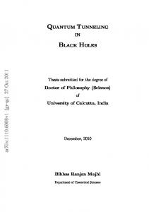
Fig. 2: (Color online) Overlaps between the initial state, Ψ0 , ˜ k of the original three-body Hamiltoand the eigenfunctions Ψ ˜k . The nian as a function of the corresponding eigenenergies, E solid and the dashed lines correspond to the cases of g = 20 and 0 MeV · fm, respectively. Notice that the initial state is the lowest eigenstate of the modified Hamiltonian, Hmod , with the eigenenergy of 4.56 MeV (5.42 MeV) for g = 20 MeV · fm (g=0 MeV · fm).

tion with the eigenfunctions of the modified Hamiltonian, that is, Ψk (x1 , x2 ) given in Eq.(11), as X Ψ(t, x1 , x2 ) = ck (t)Ψk (x1 , x2 ), (17) k

with the initial condition of ck (t = 0) = δk,0 .

(18)

Survival Probability

4

Substituting Eq. (17) into (15) and using the orthogonality of Ψk , we obtain the differential equation for the expansion coefficients ci (t),

k

Using the wave function so obtained, one can compute the survival probability, Ps (t), and the decay width, Γ, as [34–38], 2

2

Ps (t) ≡ |hΨ0 |Ψ(t)i| = |c0 (t)| , P˙ s (t) . Γ = −~ Ps (t)

(21)

A.

RESULTS

Decay energy and width

Before we numerically solve the time-dependent Schr¨odinger equation, let us first investigate the overlaps between the initial wave function Ψ0 and the eigenfunctions of the original Hamiltonian H. That is, ˜ k |Ψ0 i|2 , Qk ≡ |hΨ

(23)

˜ k i is the eigenfunctions of the original Hamiltowhere |Ψ nian satisfying ˜ ki = E ˜ k |Ψ ˜ k i. H|Ψ

(b)

g=0 (MeV fm) g=4 (MeV fm) g=18 (MeV fm) g=32 (MeV fm)

1 0.9 0.8 0.7 0.6

10

-2

8 6 4 2 0 0

200 400 600 800 1000 1200 1400 t (fm/c)

(22)

When the survival probability is an exponential function of t, the decay width Γ becomes a constant. In the next section, we will show that Ps (t) indeed has an exponential form after a sufficient time evolution. III.

g=0 (MeV fm) g=4 (MeV fm) g=18 (MeV fm) g=32 (MeV fm)

0.5

Γ (10 MeV)

dci (t) i~ = hΨi | H | Ψi (19) dt X = ck (t) (Ei δi,k + hΨi | ∆V | Ψk i) . (20)

(a)

(24)

˜k for Figure 2 shows the overlaps Qk as a function of E g=0 and 20 MeV·fm. The initial state is fragmented over several eigenfunctions of the original Hamiltonian, and thus forms a wave packet which evolves in time. As one can see, the fragmentation of the initial state is small, where the energy spreading corresponds to the decay width. Let us now numerically solve the time-dependent Schr¨odinger equation. To this end, we use a time mesh of ∆t = 0.01 fm/c. Fig.3 shows the survival probability

Fig. 3: (Color online) (a) The survival probability as a function of time t defined by Eq.(21). (b) The decay width defined by Eq.(22). These are plotted for several values of g indicated in the figure.

and the decay width defined as Eqs. (21) and (22) as a function of time t for several values of g. One can see that the decay width converges to a constant value after sufficient time-evolution, that indicates the exponential decay-law, Ps (t) = e−iΓt/~ . Notice that the converged values for the decay width with this model Hamiltonian are in the same order as the experimental width for 6 Be and 16 Ne [19–21, 54]. At shorter period, the decay width shows a transient behaviour [34–38]. That is, the survival probability behaves like a parabolic function of t, whereas the decay width increases linearly [55]. The dependence of the decay width on the strength of the pairing interaction is shown in Fig. 4 (b). We also show in Fig. 4 (a) the decay energy E0 (that is, the eigenenergy of the modified Hamiltonian given by Eq. (10)) and the asymptotic kinetic energy of diproton, Erel , defined as Erel = E0 + Bpp ,

(25)

where Bpp = mg 2 /4~2 is the binding energy of a diproton. The decay width is estimated at t = 1200 fm/c, where it has been well converged (see Fig. 3). The decay width Γ first decreases as a function of g, despite that the diproton kinetic energy Erel increases. This should be related to the decrease of the decay energy E0 , indicating that the sequential two-proton emissions is the main decay mechanism in this region of g even

5 E0 Erel

-2

-3

8.0×10

-4

6.0×10

-4

4.0×10

-4

-32

2.0×10

-4

-48

0.0×10

0

1.0×10

-3

32

8.0×10

-4

16

6.0×10-4

x2 (fm)

32 16 0

-16

(b) Γ (10 MeV)

(a) t=0 (fm/c) 1.0×10

48

8 7 6 5 4 3 2 1

-48 -32 -16 0 16 32 48 x1 (fm)

48

0

4

8

12

16

20

24

28

32

g (MeV fm)

x2 (fm)

Energy (MeV)

(a) 11 10 9 8 7 6 5 4 3

(b) t=300 (fm/c)

0

4.0×10-4

-16

Fig. 4: (Color online) (a) The decay energy E0 of the threebody system as a function of the strength of the pairing interaction, g. The dashed line indicates the asymptotic kinetic energy of a bound diproton. (b) The decay width estimated at t = 1200 fm/c.

-32

2.0×10-4

-48

0.0×100

though two protons are bound in this one-dimensional model. For g ≥ 18 MeV·fm, on the other hand, the decay width increases. This is consistent with the increase of Erel , suggesting that the direct diproton decay, that is the emission of a deeply bound diproton, is the main mechanism in this region. The transition from the sequential to the diproton decays will be clarified more in the next subsection.

48

x2 (fm)

-48 -32 -16 0 16 32 48 x1 (fm) (c) t=600 (fm/c)

32

8.0×10-4

16

6.0×10-4

0

4.0×10-4

-16

2.0×10-4

-32

0.0×100

-48

B.

Two-particle density and flux distributions

In order to confirm a transition from a sequential to a simultaneous decays discussed in the previous subsection, we next discuss the time evolution of two-particle density distribution, ρ(t, x1 , x2 ) =| Ψ(t, x1 , x2 ) |2 .

(26)

We also analyze the flux distribution defined as,   ~ ∂Ψ ∂Ψ∗ ji (t, x1 , x2 ) = Ψ∗ − Ψ (j = 1, 2). 2im ∂xi ∂xi (27) Note that the 2p density is normalized as Z ∞ ρ(t, x1 , x2 )dx1 dx2 = 1. (28) −∞

Figs.5 and 6 show the two-particle density and flux distributions, respectively, for g = 20 MeV · fm at t = 0, 300

1.0×10-3

-48 -32 -16 0 16 32 48 x1 (fm)

Fig. 5: (Color online) The time-evolution of the density distribution ρ(t, x1 , x2 ) in the two-dimensional (x1 , x2 ) plane calculated with the pairing strength of g=20 MeV · fm. The panels (a), (b), and (c) correspond to the density at t = 0, 300, and 600 fm/c, respectively.

and 600 fm/c. The corresponding quantities for g = 0 are also shown in Figs.7 and 8. The flux distributions are plotted in a form of vector at each value of (x1 , x2 ) in the two-dimensional (x1 , x2 ) plane, where the core nucleus is located at the origin. Note that there is no flux distribution at t = 0 because the initial wave function Ψ(t = 0) can be taken to be real, and we do not show it in the figures. Figs. 5(a) and 7(a) show the density distribution for

6

48

32

32

16

16

x2 (fm)

x2 (fm)

(a) t=300 (fm/c) 48

0

1.0×10

-3

8.0×10

-4

6.0×10

-4

4.0×10

-4

0

-16

-16 -32

2.0×10

-4

-32

-48

0.0×10

0

1.0×10

-3 -4

-48 -48 -32 -16 0 16 32 48 x1 (fm)

-48 -32 -16 0 16 32 48 x1 (fm)

(b) t=600 (fm/c)

(b) t=300 (fm/c)

48

32

32

8.0×10

16

16

6.0×10-4

0

x2 (fm)

48

0

4.0×10-4

-16

-16

-32

-32

2.0×10-4

-48

0.0×100

-48 -48 -32 -16 0 16 32 48 x1 (fm)

Fig. 6: (Color online) The flux distributions j(t, x1 , x2 ) = j1 (t, x1 , x2 )e1 + j2 (t, x1 , x2 )e2 , where ei is the unit vector in the two-dimensional (x1 , x2 ) plane. These are obtained with g=20 MeV · fm at t= 300 fm/c (Fig. 6(a)) and 600 fm/c (Fig. 6(b)), and are plotted in arbitrary units.

-48 -32 -16 0 16 32 48 x1 (fm)

48

x2 (fm)

x2 (fm)

(a) t=0 (fm/c)

(c) t=600 (fm/c)

32

8.0×10-4

16

6.0×10-4

0

4.0×10-4

-16

the initial 2p state, which is confined within the modified potential, Vmod . Because of the pairing correlation, the initial density for g = 20 MeV · fm has an asymmetric form, with the peaks along x1 = x2 being higher than those along x1 = −x2 [41]. The peaks along the x1 = x2 line, that is, in the first and third quadrants of these panels, correspond to a compact diproton cluster. On the other hand, the peaks along the x1 = −x2 line (i.e., in the second and the fourth quadrants) correspond to a configuration in which two protons are located opposite to the core nucleus. If we discard the pairing interaction, the density distribution has four symmetric peaks, as shown in Fig. 7, that is, the probability in the first and third quadrants is the same as that in the second and fourth quadrants [41]. The effect of pairing correlation is apparent also during the time evolution. In the presence of the pairing correlation, the extension of the two-particle density along the x1 = x2 line increases significantly, although the extension along the x1 = 0 or x2 = 0 lines is not negligible. This is in marked contrast with the uncorrelated case shown in Fig. 7, in which the two-particle density expands democratically. That is, in the uncorrelated case,

1.0×10-3

2.0×10-4

-32

0.0×100

-48 -48 -32 -16 0 16 32 48 x1 (fm)

Fig. 7: (Color online) Same as Fig.5, but for g=0 MeV · fm.

the probability of emission of the two protons in opposite directions is equal to that in the same direction. The flux distribution shown in Figs. 6 and 8 also indicate the same behaviour. In order to investigate the time evolution more quantitatively, we divide the (x1 , x2 ) plane into four regions shown in Fig. 9. That is, (i) the region of x1 > 16 fm and x2 > 16 fm, as well as the region of x1 < −16 fm and x2 < −16 fm, (ii) the region of x1 > 16 fm and x2 < − 16 fm, as well as the region of x1 < −16 fm and x2 > 16 fm, (iii) the region of −16 ≤ x1 ≤ 16 fm and |x2 | > 16 fm, as well as the region of −16 ≤ x2 ≤ 16 fm and |x1 | > 16 fm, and (iv) the rest in the (x1 , x2 ) plane. At each time,

7

(a) t=300 (fm/c) 48

x2

x2 (fm)

32

16 fm

ղ ճ ձ

16 0

ճ մ ճ x

-16

1

-32 -48 -48 -32 -16 0 16 32 48 x1 (fm)

ձ ճ ղ

(b) t=600 (fm/c) 48

x2 (fm)

32 16 0 -16

Fig. 9: (Color online) The four regions in the (x1 , x2 ) plane used to calculate the partial probabilities shown in Fig. 10. The boundaries of each region are at x1 = ±16 fm and x2 = ±16 fm.

-32 -48 -48 -32 -16 0 16 32 48 x1 (fm)

Fig. 8: (Color online) Same as Fig.6, but for g=0 MeV · fm.

we integrate the two-particle density distribution in each region, Z ρ(t, x1 , x2 )dx1 dx2 , (k = 1 ∼ 4). (29) Pk (t) = region k

The time evolution of these partial probabilities is shown in Fig.10 for g = 0, 20 and 32 MeV ·fm. We also show the total decay probability, that is, 1 − P4 = P1 + P2 + P3 . We first discuss the behaviour for the uncorrelated case shown in Fig. 10 (a). In this case, the dominant process is the decay into the third region, P3 , which corresponds to an emission of one of the valence protons while the other proton remains inside the core-proton potential. As there is no active s.p. bound state in the present core-proton potential, the second proton mainly occupies the s.p. resonance state. This resonance state eventually decays and the second proton is emitted outside the potential after a sufficient time-evolution. This is nothing but the sequential two-proton decay, and can be clearly seen in the probabilities P1 and P2 , that exist only at t & 600 fm/c. Notice that P1 and P2 are identical to each other, since the second proton is emitted into either the left or the right direction with respect to the core nucleus with an equal probability irrespective to the position of the first proton. For g = 20 MeV · fm shown in Fig. 10(b), the proba-

bility in the region (i) increases considerably due to the pairing correlation, while P3 decreases significantly. This partly corresponds to an emission of a bound diproton, that is, the simultaneous two-proton decay. Notice, however, that P3 is still larger than P1 at t . 800 fm/c, and a sequential decay also coexists for this value of g. As we have shown in Fig.4, the total decay probability, P1 + P2 + P3 , decreases compared to the uncorrelated case. When the pairing interaction is even stronger, the simultaneous diproton decay becomes dominant. See Fig.10 (c) for g = 32 MeV · fm. In this case, P1 is the dominant part of the total decay probability, except for the short time region, at which the high energy components in the initial wave function quickly escape from the potential barrier. The long-time behaviour in this case may correspond to alpha decays in realistic nuclei, for which a tightly bound alpha particle tunnels through the Coulomb barrier of the daughter nucleus. From these studies, it is evident that the present onedimensional three-body model nicely describes a transition from an uncorrelated case to a strongly correlated case for many-particle tunneling decays. IV.

SUMMARY

We have employed the time-dependent method and investigated many-particle tunneling decays, particularly the two-proton radioactivity. To this end, we have used a one-dimensional three-body model which consists of a core nucleus and two valence protons. In order to describe the decaying process, we first confined the twoproton wave function inside a confining potential. The confining potential was then changed to the original po-

8 0.4 (a) g=0 (MeV fm)

Pk

0.3 0.2

P1 P2 P3 1-P4

0.1

Pk

0 (b) g=20 (MeV fm)

0.1 0 0.4

(c) g=32 (MeV fm)

Pk

0.3 0.2 0.1 0 0

200 400 600 800 1000 1200 1400 t (fm/c)

time evolution of the density and flux distributions. We have also analyzed the partial probabilities and discussed the relative importance of the sequential and simultaneous two-proton decays. We have shown that, for the uncorrelated case, the sequential decay is the dominant decay process, while the simultaneous decay plays an essential role in the case of strong pairing correlation. For an intermediate value of the pairing strength, we have shown that both the simultaneous and the sequential two-proton emission coexist. The one-dimensional three-body model which we employed in this paper is a simple schematic model, with which a deep understanding of many-particle decay process may be obtained. One drawback, however, is that two protons are inevitably bound even with an infinitesimal attraction between the two protons. Even though our model nicely demonstrates the coexistence of the simultaneous and sequential decays for an intermediate pairing interaction, in reality two protons are never bound in vacuum. It will be an important task to extend the present study to realistic two-proton emitters in three-dimension, such as 6 Be and 16 Ne nuclei. A work towards this direction is in progress, and we will report on it in a separate publication.

Fig. 10: (Color online) The time-evolution of the partial probabilities in the regions defined in Fig. 9 for g=0, 20, and 32 MeV·fm. The total decay probability, Ptot ≡ 1 − P4 = P1 + P2 + P3 , is also shown by the dot-dashed lines.

Acknowledgments

tential, with which the two-proton wave function evolves in time. We have confirmed that the survival probability follows the exponential decay-law after a sufficient time-evolution, yielding a constant decay width. We have found that an emission of a bound diproton is enhanced due to the pairing correlation, as was evidenced in the

We thank D. Lacroix for useful discussions. This work was supported by the Global COE Program “Weaving Science Web beyond Particle-Matter Hierarchy” at Tohoku University, and by the Japanese Ministry of Education, Culture, Sports, Science and Technology by Grantin-Aid for Scientific Research under the program number (C) 22540262.

[1] J. Bardeen, Phys. Rev. Lett. 6, 57 (1961). [2] C.A. Caldeira and A.J. Leggett, Ann. of Phys. (N.Y.) 149, 374 (1983). [3] V. V. Flambaum and V. G. Zelevinsky, J. Phys. G 31, 335 (2005). [4] C. A. Bertulani, V. V. Flambaum and V. G. Zelevinsky, J. Phys. G 34, 2289 (2007). [5] N. Ahsan and A. Volya, Phys. Rev. C 82, 064607 (2010). [6] A. C. Shotter and M. D. Shotter, Phys, Rev. C 83, 054621 (2011). [7] A.B. Balantekin and N. Takigawa, Rev. Mod. Phys. 70, 77 (1998). [8] M. Dasgupta, D.J. Hinde, N. Rowley and A.M. Stefanini, Annu. Rev. Part. Sci. 48, 401 (1998). [9] R. Vandenbosch and J.R. Huizenga, Nuclear Fission (Academic Press Inc., 1974). [10] D.S. Delion, Theory of particle and cluster emission (Springer-Verlag, Berlin, 2010). [11] C.A. Bertulani and P. Danielewicz, Introduction to nu-

clear reactions (Institute of Physics Publishing, London, 2004). I.J. Thompson and F.M. Nunes, Nuclear reactions for astrophysics (Cambdridge University Press, Cambridge, 2009). K. Sasaki, K, Suekane and I. Tonozuka, Nucl. Phys. A 147, 45 (1970). I. Tonozuka and A. Arima, Nucl. Phys. A 323, 45 (1979) K. Varga and R.J. Liotta, Phys. Rev. C 50, R1292 R1295 (1994) M. Pfutzner et al., Eur. Phys. J. A. 14, 279 (2002). J. Giovinazzo et al., Phys. Rev. Lett. 89, 102501 (2002). K. Miernik et al., Phys. Rev. Lett. 99, 192501 (2007). O.V.Bochkarev et al., Nucl. Phys. A 505, 215 (1989). L. V. Grigorenko et al., Phys. Rev. C 64, 054002 (2001). L. V. Grigorenko et al., Phys. Rev. C 80, 034602 (2009). M. Pf¨ utzner, M. Karny, L.V. Grigorenko, and K. Riisager, Rev. Mod. Phys., in press. e-print: arXiv:1111.0482v1 [nucl-ex].

[12] [13] [14] [15] [16] [17] [18] [19] [20] [21] [22]

9 [23] B. Blank and M. Ploszajczak, Rep. Prog. Phys. 71 (2008) 046301. [24] L.V. Grigorenko, Phys. of Part. and Nucl. 40 (2009) 674, and references therein. [25] L.V. Grigorenko, T.D. Wiser, K. Mercurio, R.J. Charity, R. Shane, L.G. Sobotka, J.M. Elson, A.H. Wuosmaa, A. Banu, M. McCleskey, L. Trache, R.E. Tribble, and M.V. Zhukov, Phys. Rev. C80 (2009) 034602. [26] M. Matsuo, K. Mizuyama and Y. Serizawa, Phys. Rev. C 71, 064326 (2005). [27] M. Matsuo, Phys. Rev. C 73, 044309 (2006). [28] K. Hagino and H. Sagawa, Phys. Rev. C 72, 044321 (2005). [29] T. Oishi, K. Hagino and H. Sagawa, Phys. Rev. C 82, 024315 (2010). [30] A. Spyrou et al., Phys. Rev. Lett. 108, 102501 (2012). [31] M. Grasso, D. Lacroix and A. Vitturi, Phys, Rev. C 85, 034317 (2012). [32] G. Scamps, D. Lacroix, G. F. Bertsch and K. Washiyama, Phys, Rev. C 85, 034328 (2012). [33] G. Potel et al., Phys. Rev. Lett. 105, 172502 (2010); Phys. Rev. Lett. 107, 092501 (2011). [34] O. Serot, N. Carjan and D. Strottman, Nucl. Phys. A 569, 562 (1994). [35] P. Talou, N. Carjan and D. Strottman, Phys. Rev. C 58, 3280 (1998). [36] P. Talou, N. Carjan and D. Strottman, Nucl. Phys. A 647, 21 (1999). [37] P. Talou, D. Strottman and N. Carjan, Phys. Rev. C 60, 054318 (1999). [38] P. Talou et al., Phys. Rev. C 62, 014609 (2000).

[39] Gast´ on Garc´ıa-Calder´ on and Luis Guilllermo MendozaLuna, Phys. Rev. A 84, 032106 (2011). [40] C.N. Davids and H. Esbensen, Phys. Rev. C61, 054302 (2000). [41] K. Hagino et al., J. Phys. G 38, 015105 (2011). [42] M.S. Pindzola, D.C. Griffin, and C. Bottcher, Phys. Rev. Lett. 66, 2305 (1991). [43] R. Grobe and J.H. Eberly, Phys. Rev. Lett. 68, 2905 (1992); Phys. Rev. A48, 4664 (1993). [44] M. Lein, E.K.U. Gross, and V. Engel, Phys. Rev. Lett. 85, 4707 (2000). [45] T. Oishi, K. Hagino, and H. Sagawa, Phys. Rev. C84, 057301 (2011). [46] H. Nakada and M. Yamagami, Phys. Rev. C83, 031302(R) (2011). [47] E. Merzbacher, Quantum Mechanics, 3rd ed. (John Wiley & Sons, New York, 1998); S. Gasiorowicz, Quantum Physics, 3rd ed. (John Wiley & Sons, New York, 2003). [48] S. A. Gurvitz and G. Kalbermann, Phys. Rev. Lett. 59, 262 (1987). [49] S. A. Gurvitz, Phys. Rev. A 38, 1747 (1988). [50] S. A. Gurvitz et al., Phys. Rev. A 69, 042705 (2004). [51] A. U. Hazi and H. S. Taylor, Phys. Rev. A1, 1109 (1970). [52] C. H. Maier, L. S. Cederbaum and W. Domcke, J. Phys. B 13, L119-L124 (1980). [53] Li Zhang et al., Rev. C 82, 014312 (2008). [54] I. Mukha et al., Phys. Rev. C 77, 061303(R) (2008). [55] K. Grotz and H. V. Klapdor, Phys. Rev. C 30, 2098 (1984).