network, each non-terminal node of a DD is realized by a multi- plexer (MUX). We propose heuristic algorithms to derive SMT-. MDDs from SBDDs. We compare ...
IEICE TRANS. INF. & SYST., VOL.E82–D, NO.5 MAY 1999
925
PAPER
Special Issue on Multiple-Valued Logic and Its Applications
Time-Division Multiplexing Realizations of Multiple-Output Functions Based on Shared Multi-Terminal Multiple-Valued Decision Diagrams Hafiz Md. HASAN BABU† , Nonmember and Tsutomu SASAO† , Member
SUMMARY This paper considers methods to design multiple-output networks based on decision diagrams (DDs). TDM (time-division multiplexing) systems transmit several signals on a single line. These methods reduce: 1) hardware; 2) logic levels; and 3) pins. In the TDM realizations, we consider three types of DDs: shared binary decision digrams (SBDDs), shared multiple-valued decision diagrams (SMDDs), and shared multiterminal multiple-valued decision diagrams (SMTMDDs). In the network, each non-terminal node of a DD is realized by a multiplexer (MUX). We propose heuristic algorithms to derive SMTMDDs from SBDDs. We compare the number of non-terminal nodes in SBDDs, SMDDs, and SMTMDDs. For nrm n, log n, and for many other benchmark functions, SMTMDD-based realizations are more economical than other ones,√where nrm n is a (2n)input (n+1)-output function computing � X 2 + Y 2 +0.5�, log n (2n −1) log(x+1) is an n-input n-output function computing � �, and n log 2 �a� denotes the largest integer not greater than a. key words: multiple-valued decision diagram (MDD), multiplevalued logic, multiple-output function, time-division multiplexing (TDM)
1.
In the network, each non-terminal node of a decision diagram (DD) is realized by a multiplexer (MUX). The rest of the paper is organized as follows: Section 2 defines various DDs for multiple-output functions. Section 3 shows TDM realizations of multiple-output functions based on SBDDs, SMDDs, and SMTMDDs. Section 4 presents methods to derive SMTMDDs from SBDDs. Section 5 shows upper bounds on the size of an SBDD and an SMTMDD to represent an n-input moutput function. Experimental results for arithmetic functions and other benchmark functions are shown in Sect. 6. 2.
Decision Diagrams Functions
for
Multiple-Output
In this section, we show three different decision diagrams to represent multiple-output functions.
Introduction 2.1 Shared Binary Decision Diagrams
In modern LSIs, one of the most important issue is the “pin problem.” The reduction of the number of pins in the LSIs is not so easy, even though the integration of more gates may be possible. To overcome the pin problem, the time-division multiplexing (TDM) systems are often used. In the TDM system, a single signal line represents several signals. For example, the Intel 8088 microprocessors used 8-bit buses to represent 16-bit data which made it possible to produce a large amount of microcomputers so quickly while the 16-bit peripheral LSIs were not so popular in the early 1980s. In this paper, we present a method to design multiple-output networks based on shared multi-terminal multiple-valued decision diagrams (SMTMDDs) by using TDMs. We propose heuristic algorithms to derive SMTMDDs from shared binary decision diagrams (SBDDs), and compare realizations based on SMTMDDs with the ones based on SBDDs and shared multiple-valued decision diagrams (SMDDs). Experimental results show the compactness of SMTMDDs over SBDDs and SMDDs. Manuscript received September 10, 1998. Manuscript revised November 11, 1998. † The authors are with the Department of Computer Science and Electronics, Kyushu Institute of Technology, Iizuka-shi, 820–8502 Japan.
A shared binary decision diagram (SBDD) is a set of binary decision diagrams (BDDs) combined by a tree for output selection. Note that the definition of the SBDD in this paper is somewhat different from [16]. For example, Fig. 1 shows the SBDD for Table 1.
Fig. 1
SBDD for the function in Table 1.
IEICE TRANS. INF. & SYST., VOL.E82–D, NO.5 MAY 1999
926 Table 1 x1 0 0 0 0 0 0 0 0 1 1 1 1 1 1 1 1
2-valued 4-input 4-output function. Input x2 x3 0 0 0 0 0 1 0 1 1 0 1 0 1 1 1 1 0 0 0 0 0 1 0 1 1 0 1 0 1 1 1 1
x4 0 1 0 1 0 1 0 1 0 1 0 1 0 1 0 1
f0 0 1 0 1 1 0 1 1 0 1 1 0 1 0 1 0
Output f1 f2 1 1 0 1 1 0 1 1 0 0 1 1 0 1 1 0 0 0 0 1 1 0 1 1 0 0 1 1 1 1 1 0
f3 0 1 1 1 1 0 1 0 1 1 1 1 1 0 1 0
Fig. 3 Table 2
SMTMDD for the function in Table 2. 4-valued 2-input 2-output function. Input X1 X2 0 0 0 1 0 2 0 3 1 0 1 1 1 2 1 3 2 0 2 1 2 2 2 3 3 0 3 1 3 2 3 3
Fig. 2
Output Y1 Y2 1 2 2 3 1 1 3 3 2 1 1 2 2 3 3 0 0 1 2 3 3 1 1 3 2 1 1 2 3 3 1 0
SMDD for the function in Table 1.
Multi-terminal binary decision diagrams (MTBDDs) are the extended BDDs with multiple terminal nodes, where the terminals are m-bit binary vectors for m output functions. A shared multi-terminal binary decision diagram (SMTBDD) is a set of MTBDDs combined by a tree for output selection [1]–[3], [6], [7], [9], [16]. 2.2 Shared Multiple-Valued Decision Diagrams A shared multiple-valued decision diagram (SMDD) is a set of multiple-valued decision diagrams (MDDs) combined by a tree for output selection [4]. Figure 2 shows the SMDD for Table 1, where g0 , g1 , and g2 are the output selection variables, and X1 and X2 are the pairs of binary inputs. 2.3 Shared Multi-Terminal Multiple-Valued Decision Diagrams Shared multi-terminal multiple-valued decision diagrams (SMTMDDs) are another representations of multiple-valued multiple-output logic functions [4], [5],
[8], [10]–[15]. An SMTMDD is a set of multiplevalued decision diagrams (MDDs) with multiple terminal nodes combined by a tree for output selection. The number of MDDs in the SMTMDD is equal to the number of groups of output functions. Figure 3 shows the SMTMDD for Table 2, where Y1 and Y2 are the pairs of binary outputs, and X1 and X2 are the pairs of binary inputs. The advantage of SMTMDDs is that they can evaluate several output functions simultaneously. Moreover, the good grouping of output functions and good grouping of input variables produce compact SMTMDDs. Definition 1: The sizen of the DD denoted by sizen (DD), is the total number of non-terminal nodes excluding the nodes for output selection variables. Example 1: The sizen s of the SBDD, SMDD, and SMTMDD in Figs. 1, 2, and 3 are 19, 11, and 9, respectively. Note that g0 , g1 , and g2 are the output selection variables in the SBDD and SMDD, and g0 is the output selection variable in the SMTMDD. ✷
HASAN BABU and SASAO: TDM REALIZATIONS BASED ON SMTMDDS
927
Fig. 4
3.
TDM realization based on the SBDD.
TDM Realizations
The TDM realization uses clock pulse to reduce the number of input and output pins. On the other hand, the non-TDM realization means a conventional combinational network without using clock pulse. In this section, we will show TDM realizations of multiple-output functions based on SBDDs, SMDDs, and SMTMDDs. 3.1 TDM Realizations Based on SBDDs In this part, we introduce a method to realize multipleoutput functions by using TDM. To illustrate it, we use an example of the 4-input 4-output function shown in Table 1. Figure 4 shows a TDM realization. In the main LSI, pairs of logic functions are multiplexed by the clock pulse η. The output signals of the main LSI denote the functions as follows: G0 = η¯f0 ∨ ηf1 , and G1 = η¯f2 ∨ ηf3 . These mean when η = 0, G0 and G1 represent f0 and f2 , respectively. On the other hand, when η = 1, G0 and G1 represent f1 and f3 , respectively. In this realization, we need the hardware for the functions f0 , f1 , f2 , and f3 , as well as the hardware for multiplexing. By using this technique, we can reduce the number of output pins into a half. Note that in this example, only two lines are necessary between the main LSI and the peripheral LSI. In the peripheral LSI, we need delay latches. When η = 0, the values for f0 and f2 are transferred to the first and the third latches, respectively. On the other hand, when η = 1, the values for f1 and f3 are transferred to the second and fourth latches, respectively. To realize the multiple-output function, we use an SBDD. By replacing each non-terminal node of an SBDD by a multiplexer, we obtain a network for the multiple-output function. In this case, the amount of hardware for the network is easily estimated by the size n of the SBDD, and the design of the network is quite easy.
Fig. 5
TDM realization based on the SMTMDD.
3.2 TDM Realizations Based on SMDDs In Fig. 4, if we realize the multiple-output function by an SMDD, we have the TDM realization based on SMDDs. Each non-terminal node of an SMDD is realized by a 2-MUX in Fig. 6. Figure 7 shows the literal generator whose inputs are a pair of 2-valued variables (details will be shown in Sect. 3.3). In this method, the input variables are partitioned into pairs to make 4-valued variables, and we consider the realization of a 4-valued input 2-valued output function: Qn → B m , where Q = {00, 01, 10, 11} and B = {0, 1}. The numbers of nodes in an SMDD can be reduced as follows: • By finding the best pairing of the input variables to make 4-valued variables. • By finding the best ordering of the 4-valued variables. 3.3 TDM Realizations Based on SMTMDDs The TDM realization based on SMTMDDs is shown in Fig. 5. In this method, 4-valued logic is used instead of 2-valued logic. Consider a 2-valued multiple-output function. First, partition the input variables into pairs. For example, the input variables {x1 , x2 , x3 , x3 } in Table 1 are partitioned into X1 = (x1 , x2 ) and X2 = (x3 , x4 ). Second, partition the output functions into pairs. For example, the output functions {f0 , f1 , f2 , f3 } in Table 1 are partitioned into G0 = (f0 , f1 ) and G1 = (f2 , f3 ). Then, we have a 4-valued logic function: Q2 → Q, where Q = {0, 1, 2, 3}, as shown in Table 2. The output functions Y1 and Y2 in Table 2 correspond to G0 and G1 , respectively. In general, a 4-valued ninput m-output function: Qn → Qm is represented by an SMTMDD. Next, consider the hardware realization of an SMTMDD. Each non-terminal node of an SMTMDD is realized by a 2-MUX shown in Fig. 6. It is a 4-way multiplexer. Figure 7 shows the literal generator whose inputs are a pair of 2-valued variables (x1 , x2 ), and outputs are X 0 , X 1 , X 2 , and X 3 that control the 2-MUX. Note that
IEICE TRANS. INF. & SYST., VOL.E82–D, NO.5 MAY 1999
928
Fig. 6
2-MUX.
Fig. 8 TDM realization of a 4-output function based on the SMTMDD.
number of nodes in an SMTMDD can be reduced as follows: • By finding the best pairing of the input variables to make 4-valued variables. • By finding the best pairing of the output functions to make 4-valued functions.
Fig. 7
Xi =
�
Literal generator.
0 if X = � i, 1 if X = i.
A signal in the terminal node is represented by a pair of bits (c0 , c1 ) as follows: When η = 0, the signal represents c0 . When η = 1, the signal represents c1 . Thus, (c0 , c1 ) = (0, 0) (c0 , c1 ) = (0, 1) (c0 , c1 ) = (1, 0) (c0 , c1 ) = (1, 1)
corresponds corresponds corresponds corresponds
to to to to
a constant 0. η. η¯. a constant 1.
Figure 8 shows the SMTMDD-based TDM realization for the function in Table 2. In the inputs, a pair of 2-valued variables X = (x1 , x2 ) represents a 4-valued signal {00, 01, 10, 11} or {0, 1, 2, 3}. On the other hand, 0, η, η¯, and 1, represent (0, 0), (0, 1), (1, 0), and (1, 1), respectively. Note that {0, η, η¯, 1} constitutes the 4element Boolean algebra. If we replace {0, η, η¯, 1} by {0, 1, 2, 3}, then we have the 4-valued function in Table 2. An arbitrary 4-valued function is represented by an SMTMDD. The amount of hardware for the network is estimated by the size n of the SMTMDD. The
3.4 Comparison of TDM Realizations In this part, we compare the DD-based TDM realizations of an n-input m-output function F . In the hardware realization, each non-terminal node of a BDD is realized with two MOS transistors, while each nonterminal node of an MDD is realized with four MOS transistors. So, if we ignore the cost of literal generators, then the cost of a non-terminal node of an MDD is twice the cost of a non-terminal node of the BDD. Therefore, when (2size n (MDD : F ) < size n (BDD : F )), the MDD-based realizations are more economical than BDD-based ones. In addition, in the case of an n-variable function, a BDD-based realization requires n levels, while an MDD-based realization requires only n 2 levels. In the FPGAs, the delay of interconnections between the modules is often greater than the delay of logic modules. Thus, the reduction of logic level is important. So, MDD-based realizations can be faster and require smaller amount of hardware than BDD-based ones. 4.
Reduction of SMTMDDs
The reduction of sizen for SMTMDDs is important to design compact logic networks. We consider the following methods for reduction: 1) pairing of output functions; 2) pairing of input variables; and 3) ordering of group of input variables. The SMTBDDs
HASAN BABU and SASAO: TDM REALIZATIONS BASED ON SMTMDDS
929
are derived from the SBDDs by pairing the output functions, and the SMTMDDs are derived from the SMTBDDs by pairing the input variables. Since an SMTBDD consists of MTBDDs, and each MTBDD represents a pair of output functions, we used the following heuristics to pair the outputs: Pair output functions so that the upper bounds on the size of the MTBDD are minimized [9]. The MDD nodes for each pair of input variables are counted from SMTBDDs as follows: Subgraphs shown in Figs. 9 (a), (b), or (c), correspond to one, two, or three MDD nodes, respectively. In Fig. 9 (a), three SMTBDD nodes are replaced by one MDD node. However, in Fig. 9 (b), the SMTBDD nodes correspond to two MDD nodes. In Fig. 9 (c), the SMTBDD nodes are replaced by three MDD nodes. Finally, SMTMDDs are optimized by using sifting algorithm [17]. 5.
Upper Bounds on the Sizen of DDs
In the design of multiple-output networks, we often have to estimate the number of MUXs to realize functions. This section shows upper bounds on the number of non-terminal nodes to represent an n-input m-output function by an SBDD and an SMTMDD. Since each non-terminal node of a DD corresponds to an MUX, the size n of the DD estimates the amount of hardware.
Fig. 9
A method replacing SMTBDD nodes by MDD nodes.
Theorem 1: Consider an n-input m-output function n
k
F . Then, size n (SBDD) ≤ min{m·(2n−k −1)+22 −2}. k=1
Theorem 2: Consider a function F : {0, 1, . . . , Let m1 be the p − 1}N → {0, 1, . . . , r − 1}m . number of groups of 2-valued functions. Then, N
size n (SMTMDD) ≤ min{m1 · k=1
pN −k −1 (p−1)
Example 2: Let n = 18, m = 20, and p = r = 4. For such a function, size n (SBDD) ≤ 2621422, and ✷ size n (SMTMDD) ≤ 218702. Note that these theorems are used in the heuristic algorithm in Sect. 4. 6.
Experimental Results
We developed C programs to build SBDDs and SMTBDDs. SMTMDDs were constructed from SMTBDDs using the method in Sect. 4, while SMDDs were constructed from SBDDs using the similar technique to Fig. 9 [4]. Tables 3, 4, and 5 compare the sizen s of SBDDs, SMDDs, and SMTMDDs for nrm n, log n, and n-bit adders, respectively, where nrm√n is a (2n)input (n + 1)-output function computing X 2 + Y 2 + 0.5 , log n is an n-input n-output function computing n log(x+1)
(2 −1) , and a denotes the largest integer n log 2 not greater than a [7]. Table 6 compares the sizen s of SBDDs, SMDDs, and SMTMDDs for other benchmark functions. The symbol “ * ” in Table 6 denotes the function with don’t cares, where the don’t cares were set to zero during the experiment. The ratio1 s showing size n s of SMDDs to SBDDs are in the column 7 of Tables 3–6, while the ratio2 s showing size n s of SMTMDDs to SBDDs are in the column 8 of Tables 3–6. The ratios in these tables show the relative
Table 3 Numbers of non-terminal nodes in SBDDs, SMDDs, and SMTMDDs to represent nrm n. Function name nrm3 nrm4 nrm5 nrm6 nrm7 average3 relative sizen
In
Out
SBDD
SMDD
6 8 10 12 14
4 5 6 7 8
45 152 471 1345 3859 1.00
25 81 241 684 1590
SMTMDD 21 70 214 618 1463
ratio1
ratio2
0.55 0.53 0.51 0.50 0.41 0.50
0.46 0.46 0.45 0.45 0.37 0.43
In: number of inputs. Out: number of outputs. size (SMDD) 1. ratio = sizen (SBDD ) ; n
2. ratio =
size n (SMTMDD) ; size n (SBDD)
3. average relative sizen =
1 N1
N1 �
k
+ rp − r}.
size n of the MDD for function i , size n of the SBDD for function i
i=1
where N1 is the total number of functions.
IEICE TRANS. INF. & SYST., VOL.E82–D, NO.5 MAY 1999
930 Table 4 Numbers of non-terminal nodes in SBDDs, SMDDs, and SMTMDDs to represent log n. Function name log 6 log 8 log 10 log 12 log 14 average3 relative sizen
In
Out
SBDD
SMDD
6 8 10 12 14
6 8 10 12 14
56 196 585 1697 4833 1.00
34 108 296 851 2365
SMTMDD 33 106 277 780 2147
ratio1
ratio2
0.60 0.55 0.50 0.50 0.48 0.52
0.58 0.54 0.47 0.45 0.44 0.49
Table 5 Numbers of non-terminal nodes in SBDDs, SMDDs, and SMTMDDs to represent n-bit adders. Function name adr3 adr4 adr5 adr6 adr7 average3 relative sizen
In
Out
SBDD
SMDD
6 8 10 12 14
4 5 6 7 8
20 29 38 47 56 1.00
8 11 14 17 20
SMTMDD 9 14 19 24 29
ratio1
ratio2
0.40 0.37 0.36 0.36 0.35 0.36
0.45 0.48 0.50 0.51 0.51 0.49
Table 6 Numbers of non-terminal nodes in SBDDs, SMDDs, and SMTMDDs to represent various benchmark functions. Function name al2 amd apex4 apex5 apla* bc0 cordic cps c432 dk17* exp* ex1010* in0 max1024 misex1 misex3 pdc prom1 prom2 rd84 rot10 sao2 shift sqr6 sqr8 ts10 x4 average3 relative sizen
In
Out
SBDD
SMDD
16 14 9 117 10 26 23 24 36 10 8 10 15 10 8 14 16 9 9 8 10 10 19 6 8 22 94
47 28 19 88 12 11 2 109 7 11 18 10 11 6 7 14 40 40 21 4 6 4 16 12 16 16 71
97 256 970 1078 102 578 75 985 1298 83 193 1410 278 301 36 542 568 1971 936 59 159 85 61 71 233 146 370 1.00
81 154 465 590 61 357 41 678 749 38 127 811 137 159 22 313 350 961 483 24 79 46 45 40 123 67 395
*function with
sizes of SMDDs and SMTMDDs to SBDDs. Note that the numbers of terminal nodes in SBDDs, SMDDs, and SMTMDDs are at most 2, 2, and 4, respectively. We
SMTMDD 77 187 516 563 66 435 30 792 731 48 105 648 169 145 24 290 326 928 465 24 55 35 47 33 130 58 506
ratio1
ratio2
0.83 0.60 0.47 0.54 0.59 0.61 0.54 0.68 0.57 0.45 0.65 0.57 0.49 0.52 0.61 0.57 0.61 0.48 0.51 0.40 0.49 0.54 0.73 0.56 0.52 0.45 1.06 0.57
0.79 0.73 0.53 0.52 0.64 0.75 0.40 0.80 0.56 0.57 0.54 0.45 0.60 0.48 0.66 0.53 0.57 0.47 0.49 0.40 0.34 0.41 0.77 0.46 0.55 0.39 1.36 0.58
don0 t cares used sifting algorithm for input variables to reduce the sizen s of DDs [17]. In addition, we used algorithms in Sect. 4 to optimize SMTMDDs. Tables 3–6 show that,
HASAN BABU and SASAO: TDM REALIZATIONS BASED ON SMTMDDS
931
in most cases, size n (SMTMDD ) < size n (SBDD), and size n (SMDD) < size n (SBDD). The exception is x4 in Table 6. Tables 3 and 4 show that, for nrm n (3 ≤ n ≤ 7), and for log n (6 ≤ n ≤ 14), size n (SMTMDD ) < size n (SMDD). These tables also show that, for nrm n (3 ≤ n ≤ 7), and for log n (10 ≤ n ≤ 14), size n (SMTMDD )